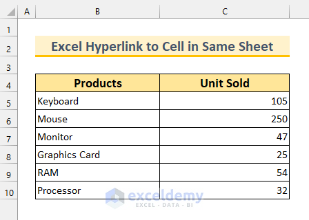
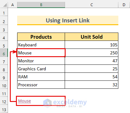
To demonstrate our methods, we’ll use the following dataset.
Method 1 – Using Insert Link Feature
Steps:
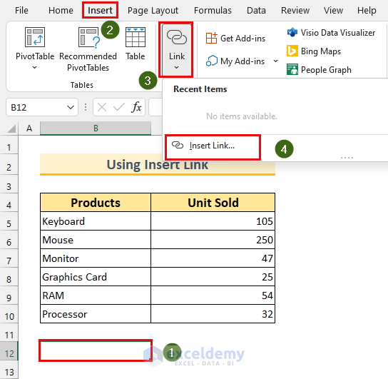
- Select cell B12.
- From the Insert tab, select Link, then Insert Link…
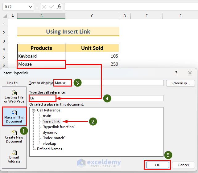
The “Insert Hyperlink” dialog box will appear.
- Select “Place in This Document”.
- Select ‘Insert link’ from “Or select a place in this document:”
- Enter “Mouse” in “Text to display:”
- Enter B6 in “Type the cell reference:”.
- Click OK.
The text “Mouse” is in cell B12 with link formatting.
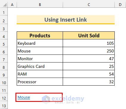
Click on it, and it will select cell B6.
Read More: How to Add Hyperlink to Another Sheet in Excel
Method 2 – Using HYPERLINK Function
Steps:
- Enter the following formula in cell B12:
=HYPERLINK("#C5","Keyboard Sold")The HYPERLINK function returns a clickable value. Here, we’ll get the link to cell C5. Moreover, we used a hash (“#”) to indicate within this Sheet. We display the second argument of the function (“Keyboard Sold”) in cell B12.
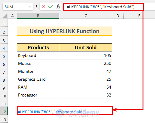
- Press ENTER.
The text “Keyboard Sold” appears in cell B12.
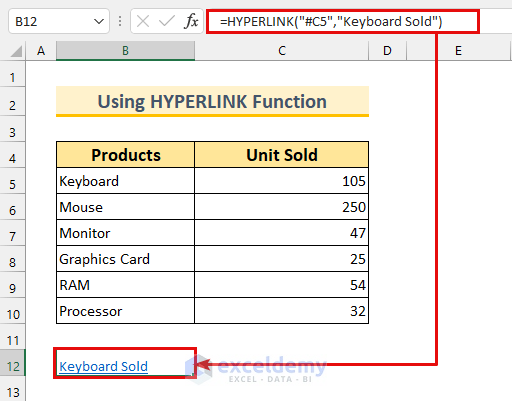
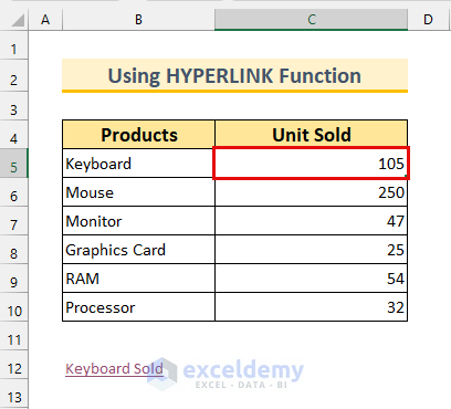
Click on this link to go to cell C5.
Read More: How to Hyperlink Multiple Cells in Excel
Method 3 – Using Combined Functions to Create Dynamic Hyperlink
For the third method, we’ll use the ADDRESS, ROW, and HYPERLINK functions to create a dynamic link to a cell in the same Sheet. This means that if we delete or insert rows or columns in the dataset, our formula will not break.
Steps:
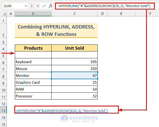
- Enter the following formula in cell B13:
=HYPERLINK("#"&ADDRESS(ROW($C8),3),"Monitor Sold")Formula Breakdown
- ADDRESS(ROW($C8),3)
- Output: {“$C$8”}.
- The ROW function returns the row number of a cell. Cell C8 will return 8. The ADDRESS function returns the location of a cell reference. Here, we’re denoting the C column by giving the value 3 in the formula.
- Our formula reduces to HYPERLINK(“#”&{“$C$8″},”Monitor Sold”)
- Output: “Monitor Sold”.
- The HYPERLINK function returns a clickable value. Here, we’ll get the link to cell C8. We use a hash (“#”) to indicate within this Sheet. We display the second argument, “Monitor Sold”, in cell B13.
- Press ENTER.
The output is as described above.
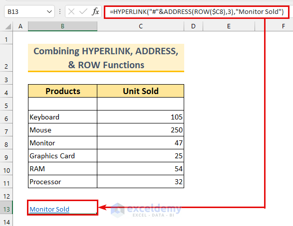
Click on that value to go to cell C8.
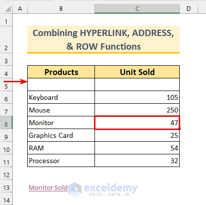
Let’s delete the blank rows to verify our dynamic formula still works.
- Remove Row 5.
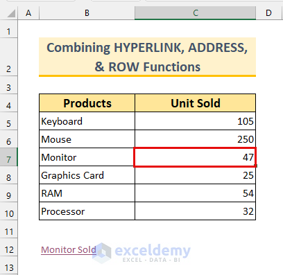
Now if we click on the text “Monitor Sold”, we move to cell C7. Therefore, our formula works flawlessly.
Read More: How to Create Dynamic Hyperlink in Excel
Method 4 – Hyperlink to First Matched Cell
Now we’ll use the CELL, INDEX, and MATCH functions to create a Hyperlink to the first matched values in the same Sheet.
Steps:
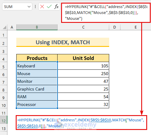
- Enter the following formula in cell B12:
=HYPERLINK("#"&CELL("address",INDEX($B$5:$B$10,MATCH("Mouse",$B$5:$B$10,0))),"Mouse")Formula Breakdown
- MATCH(“Mouse”,$B$5:$B$10,0)
- Output: 2.
- The MATCH function is used to find the position of a value. Here, we’re looking for the value “Mouse” in the cell range B5:B10. The 0 for the third argument indicates exact matching.
- Our INDEX reduces to -> INDEX($B$5:$B$10,2)
- Output: “Mouse”.
- The INDEX function returns a value from a range. Here, we get the value from the second row of the cell range B5:B10 which is cell B6.
- Our CELL formula reduces to CELL(“address”,”Mouse”)
- Output: “$B$6”.
- The CELL function returns information about a cell. Here, we’ve set info_type as “address”. This will return the first occurrence of the text “Mouse” in our range, which is cell B6.
- Our formula reduces to, HYPERLINK(“#”&”$B$6″,”Mouse”)
- Output: “Mouse”.
- The HYPERLINK function returns a clickable value. Here, we’ll get the link to cell B6. We’ve again used a hash (“#”) to indicate within this Sheet. We’ll display the second argument in cell B12, which is “Mouse”.
- Press ENTER.
The output is as described in the formula breakdown above.
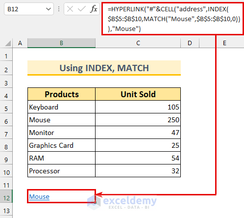
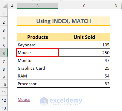
Click on the text “Mouse”, and it will select cell B6.
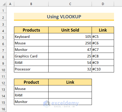
Method 5 – Creating Hyperlink to Cell in Same Sheet from a Value
Here we’ll use the HYPERLINK and VLOOKUP functions together. We’ve adjusted our dataset a bit to demonstrate the method.
Steps:
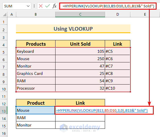
- Enter the following formula in cell C13:
=HYPERLINK(VLOOKUP(B13,B5:D10,3,0),B13&" Sold")Formula Breakdown
- VLOOKUP(B13,B5:D10,3,0)
- Output: “#C6”.
- The VLOOKUP function returns a value from a range on the left side.
- We’re looking for the value in cell B13 which is “Mouse”.
- We set our range to B5:D10.
- We’ll extract the value from column 3 which is the “Link” column.
- We use 0 to find an exact match.
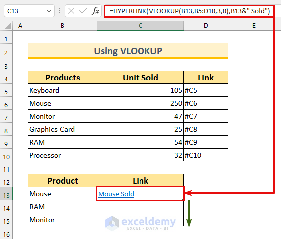
- Our formula reduces to, HYPERLINK(“#C6″,B13&” Sold”)
- Output: “Mouse Sold”.
- The HYPERLINK function returns a clickable value. Here, we’ll get the link to cell C6. There is a hash (“#”) to indicate within this Sheet. We’ll display the second argument in cell B13 joined with the text “Sold”, namely “Mouse Sold”.
- Press ENTER.
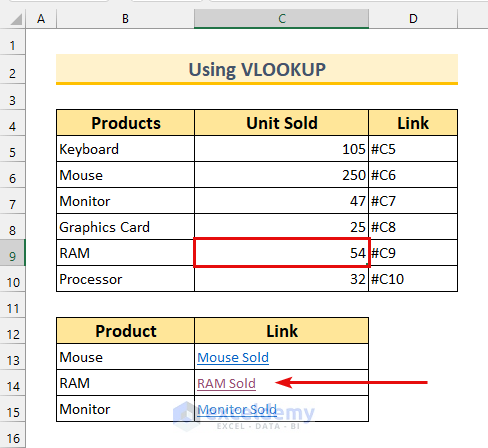
- Use the Fill Handle to AutoFill the formula.
Click on any of the Hyperlinks to go to their respective “Unit Sold” values in the dataset.
Read More: Excel Hyperlink to Cell in Another Sheet with VLOOKUP
Download Practice Workbook
Related Articles
- How to Combine Text and Hyperlink in Excel Cell
- Excel Hyperlink to Another Sheet Based on Cell Value
- How to Create a Drop Down List Hyperlink to Another Sheet in Excel
- How to Edit Hyperlink in Excel
- How to Copy Hyperlink in Excel
- How to Convert Text to Hyperlink in Excel
- How to Create Button to Link to Another Sheet in Excel
<< Go Back To Create Hyperlink in Excel | Hyperlink in Excel | Linking in Excel | Learn Excel
Get FREE Advanced Excel Exercises with Solutions!
