How to Create a Drop Down List Hyperlink to Another Sheet in Excel

In this article, we’ll show how to navigate from one sheet to another by creating a drop-down list hyperlink to another sheet in Excel. We’ll use the HYPERLINK function and a VBA code in two different methods described with examples.

How to Create a Drop Down List of Hyperlinks to Another Sheet: 2 Methods

Let’s say we have a dataset that represents sale details for the 1st three months of the year 2020 in three different sheets. We renamed the worksheets according to the month names as January, February, and March. We want to create a drop-down list that holds the sheet names and then navigate to the sheet with the selection.

1. Create a Drop Down List Hyperlink to Another Sheet Using Formula in Excel

In this method, we’ll use the HYPERLINK function to get our job done. At first, we need to create a dropdown list with the sheet names.

Step 1:

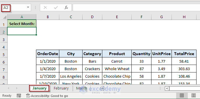
Select a cell (A2 in the worksheet named January, in this example) on which we’ll create the drop-down list.

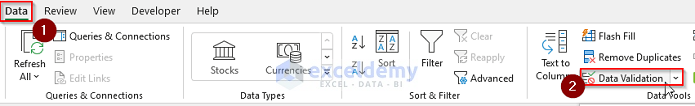
Then go to the Data tab of the Excel Ribbon.
Click on the Data Validation tab.

Step 2:

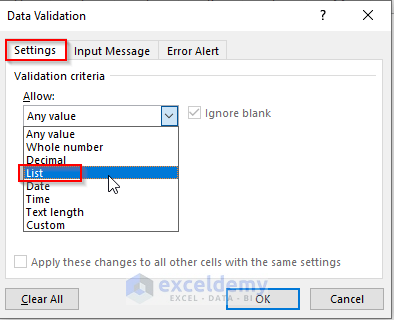
In the Data Validation window, select the Setting tab (By default selected).
In the Allow drop-down list, choose the List option.

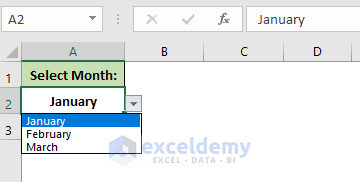
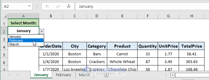
Then type January, February, and March in the Source input box and finally hit OK.
As an output, we can see a drop-down list in cell A2 with three options to select.

Step 3:

Now in cell A3, write down the following formula that uses the HYPERLINK function.

=HYPERLINK("#'" & A2 & "'!A1","Go")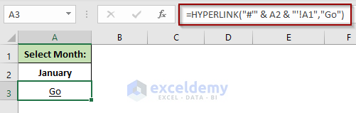

Formula Explanation:

The HYPERLINK function needs two arguments to operate. The syntax is-
=HYPERLINK(link_location,[friendly_name])
link_location – Neet to set the location that the link will take us to. In our formula–

# (pound sign) is to define that the location is within the same workbook.
A2 part takes the worksheet name from the selection in cell A2.
!A1 part determines the cell location of the selected worksheet to navigate.

The location of the link in cell A3 from the above screenshot is,
#’January’!A1
It means, clicking on the link will take us to cell A1 on the worksheet named January.
[friendly_name] – Name of the link. We set the name as “Go” in our formula.

Step 4:

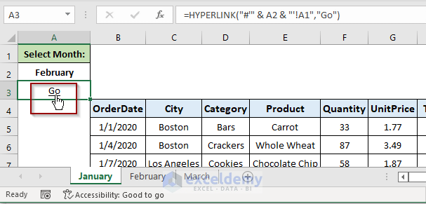
Let’s copy cells A1:A3 from the worksheet named January to other sheets named February and March. Now the drop-down list in cell A2 and the formula in cell A3 are available to all the sheets. If we want to go to sheet February from sheet January, we need to-

Select the February option from the drop-down list.

Then click on the Go link in cell A3.

We’ve successfully navigated to the sheet named February.

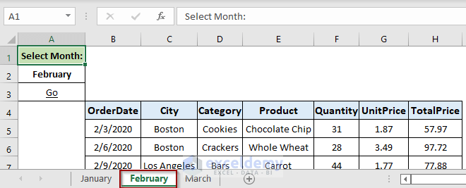
Similarly, we can choose a sheet name from the drop–down list and hit the Go link to navigate to the selected sheet.

Read More: How to Create a Hyperlink in Excel

2. Run a VBA Code to Navigate to Another Sheet Using a Drop Down List of Hyperlink in Excel

In this method, we’re going to use a VBA code to find the selected sheet name in the dropdown list and then navigate to the sheet. To illustrate this, we’ve created three new worksheets named April, May, and June.

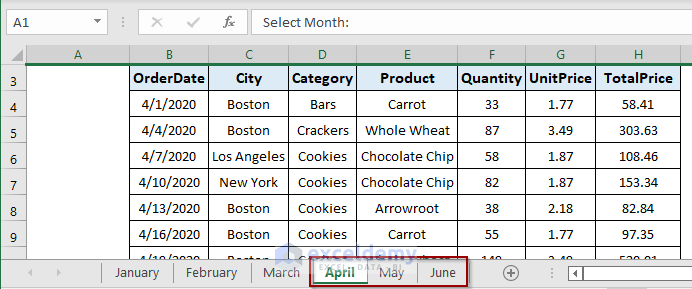
Follow the steps below:

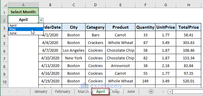
In cell A2 in the April worksheet, create a drop-down list with items April, May, and June following section 1.1.

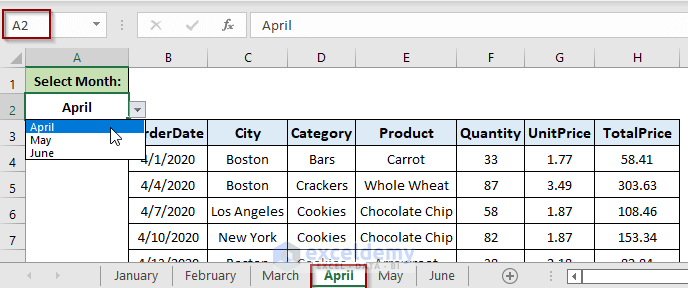
Copy the drop–down list in cell A2 to other sheets named May and June.
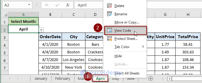
Click the right button on the sheet name and select the View Code.

Now copy and paste the following code into the visual code editor.

Private Sub Worksheet_Change(ByVal Target As Range)
    Dim SheetRng As Range, SheetName As String, TargetSheet As Worksheet
    Set SheetRng = Range("A:A")
    If Intersect(Target, SheetRng) Is Nothing Then Exit Sub
    SheetName = Target.Value
    For Each TargetSheet In Sheets
        If TargetSheet.Name = SheetName Then
            TargetSheet.Activate
        End If
    Next TargetSheet
End Sub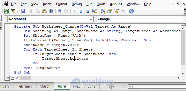

Copy and paste the same code in sheets named May and June.

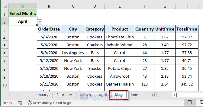
Now we can select a sheet name in the drop-down list and the code running in the background will take us to the selected worksheet. Here, we are in the sheet named April. Let’s select May from the drop-down list in cell A2.

We’ve successfully navigated to the worksheet named May automatically.

Notes

In a large dataset, we can freeze the drop–down list to facilitate the navigation to another sheet without scrolling to the top of the worksheet. To do this-

Select the third row as we want to freeze the first two rows in the worksheet named April.
Go to the View tab.
Then click on the Freeze Panes drop-down list.
Choose the Freeze Panes option.

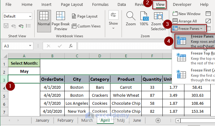
The above steps will freeze the first two rows in the worksheet.

Download Practice Workbook

Download this practice workbook to exercise while you are reading this article.

Drop Down List Hyperlink.xlsm

Conclusion

Now, we know how to navigate from one sheet to another using a drop-down list hyperlink to another sheet with examples. Hopefully, it will help you to use these methods more confidently. Any questions or suggestions don’t forget to put them in the comment box below.

<< Go Back To Excel Hyperlink to Another Sheet | Hyperlink in Excel | Linking in Excel | Learn Excel

Get FREE Advanced Excel Exercises with Solutions!