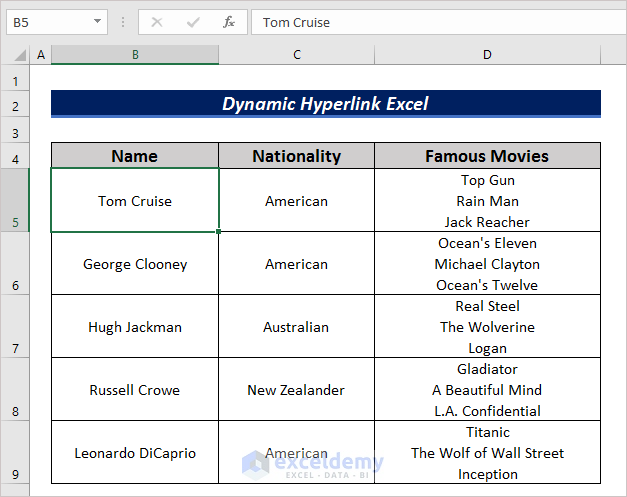
The image below is the dataset example.
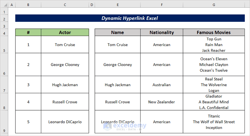
Note that this is a basic dataset to keep things simple. In a practical scenario, you may encounter a larger and more complex dataset.
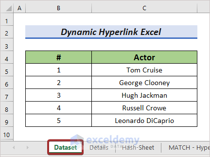
To make the examples compatible with real-life cases, let’s split the two lists into two different sheets. The Actor name list is in the Dataset worksheet.
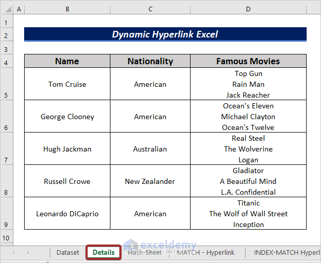
And the details in the Details worksheet.
Read More: How to Create a Hyperlink in Excel
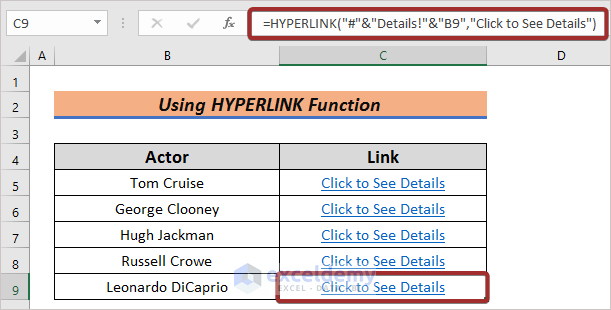
Method 1 – Use HYPERLINK Function to Create Dynamic Hyperlink
Steps:
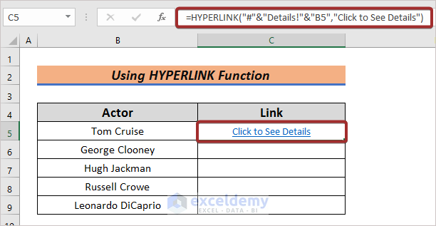
- Select a cell to create a dynamic hyperlink.
- Add the following formula in the cell to create a dynamic hyperlink.
=HYPERLINK("#"&"Details!"&"B5","Click to See Details")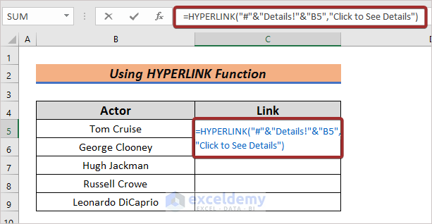
- The sheet name is Details. We have written the name followed by a “!”. Excel differentiates the sheet name and cell reference through “!”. This will generate the dynamic hyperlink.
- Click the link and it will take you to the destination cell.
- Use the AutoFill feature and generate the hyperlink for the rest of the values. But, the cell references will not be updated automatically.
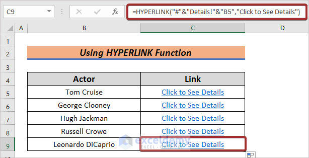
- Change the cell references manually.
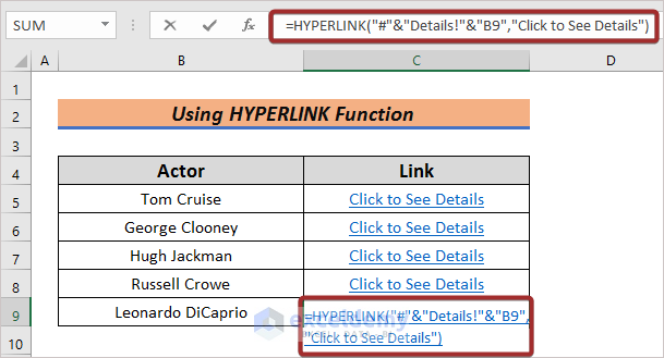
- For Leonardo DiCaprio, we have modified the cell reference to C9. This will now be linked with the correct cell.
Method 2 – Apply MATCH Function to Create Dynamic Hyperlink
Steps:
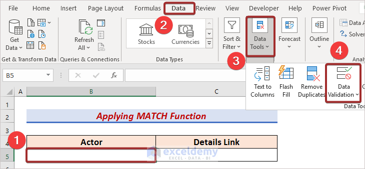
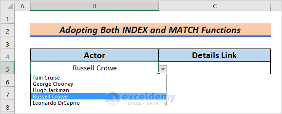
- Create a drop-down list for easing the selection of actors. For this, select a cell first to define the location of the drop-down list.
- Go to the Data tab.
- Pick Data Validation from the Data Tools tab.
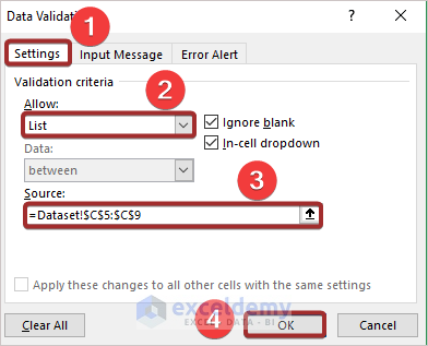
- A Data Validation wizard will pop up. Go to the Setting
- Select List in the Allow section and define the range in the Source
- Click on OK to finish the drop-down creation process.
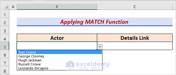
- The drop-down with the selected data can be seen.
- Input the following formula to create a dynamic hyperlink.
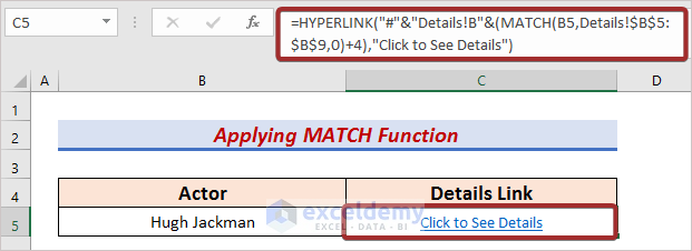
=HYPERLINK("#"&"Details!B"&(MATCH(B5,Details!$B$5:$B$9,0)+4),"Click to See Details") 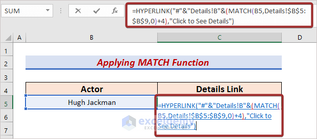
- Press the ENTER button to have a dynamic hyperlink. Click on the hyperlink and it will take you to the correct destination.
Read More: How to Activate Multiple Hyperlinks in Excel
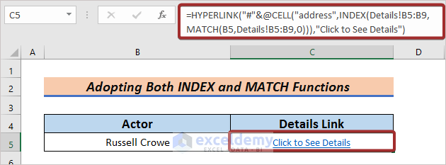
Method 3 – Combine INDEX and MATCH Functions to Create Dynamic Hyperlink
Steps:
- Generate a drop-down list first.
- Input the following formula in a cell where you want to generate a dynamic hyperlink.
=HYPERLINK("#"&CELL("address",INDEX(Details!B5:B9,MATCH(B5,Details!B5:B9,0))),"Click to See Details") 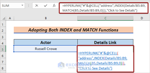
- Press ENTER to have a dynamic hyperlink. Clicking on the hyperlink will take you to the defined destination.
Read More: How to Edit Hyperlink in Excel
Download Practice Workbook
Further Readings
- How to Hyperlink to Cell in Same Sheet in Excel
- Excel Hyperlink to Cell in Another Sheet with VLOOKUP
- How to Combine Text and Hyperlink in Excel Cell
- How to Add Hyperlink to Another Sheet in Excel
- Excel Hyperlink to Another Sheet Based on Cell Value
- How to Create a Drop Down List Hyperlink to Another Sheet in Excel
- How to Copy Hyperlink in Excel
- How to Convert Text to Hyperlink in Excel
- How to Create Button to Link to Another Sheet in Excel
<< Go Back To Hyperlink in Excel | Linking in Excel | Learn Excel
Get FREE Advanced Excel Exercises with Solutions!

Dear Shakil Ahmed,
nicely mentioned, can we automate the sheet name based on a cell value? what I mean to say that as you mentioned above the cell value linked to details sheet but what would be the way to link the individual sheets based on cell value?
Hi Samad, thank you for reaching out. Fortunately there is a way to automate sheet name based on a cell value. In the image, you can see that I have a cell value in A1. I also have values in A1 cell of the other sheets. I will change the name of the corresponding sheets based on the value in A1.
Now, type the following code in a VBA module and run it.
You can see that the name of the sheet changes according to the cell value of A1. If you store sheet names in another cell such as B5, you need put this cell reference instead of A1 in the VBA code. Otherwise you will encounter errors.
So useful and clearly explained! Thanks!
Hello Ani,
You are most welcome.
Regards
ExcelDemy