How to create a Hyperlink to Another Sheet Based on the Cell Value – 4 Methods

Method 1 – Create a Hyperlink Based on Cell Value in the Context Menu in Excel

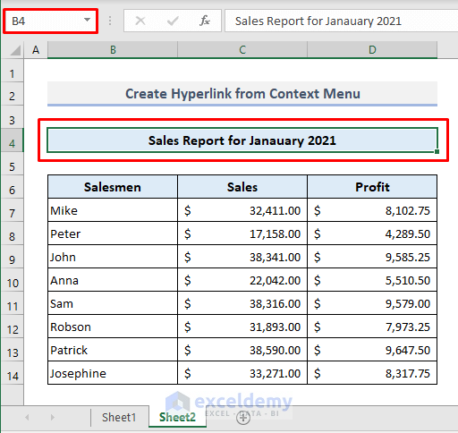
Create hyperlinks to click a month name an be redirected to the sales report of that month in another sheet (Sheet2 in January-21).

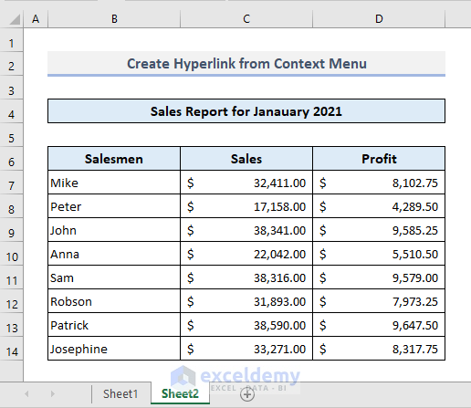
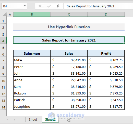
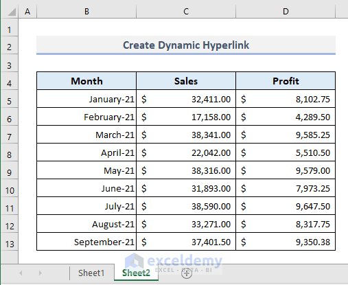
Here is Sheet2 with the sales report of January-21.

Step 1:

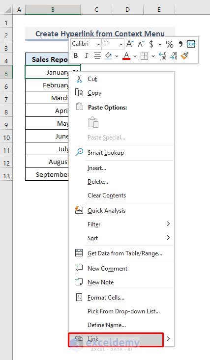
• In Sheet1, select B5.
• Right-click to open the Context Menu.
• Select Link.

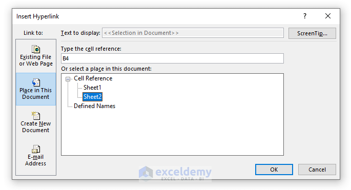
A dialog box will open.

Step 2:

• In Link to, click Place in This Document.
• In ‘Type the cell reference’, enter B4.
• Select Sheet2 in Cell Reference.
• Click OK.

The hyperlink will be added to B5 in Sheet1.

Step 3:

• Click the text in B5.

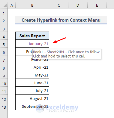
You’ll be redirected to B4 in Sheet2. Follow the same procedure to create hyperlinks for all months in Sheet1.

Read more: How to Hyperlink to Cell in Excel

Method 2 – Use the HYPERLINK function to Add a Hyperlink to Another Sheet in Excel

The generic formula of the HYPERLINK function is:

=HYPERLINK(link_location, [friendly_name])

The first argument selects the location the hyperlink will redirect you to. The Hash symbol (#) before the location keeps the search in the same workbook. The entire first argument in enclosed with Double-quotes (“ “).

The text value in the second argument is present in the cell containing the hyperlink.

Sheet1 has an additional column with the Hyperlinks header.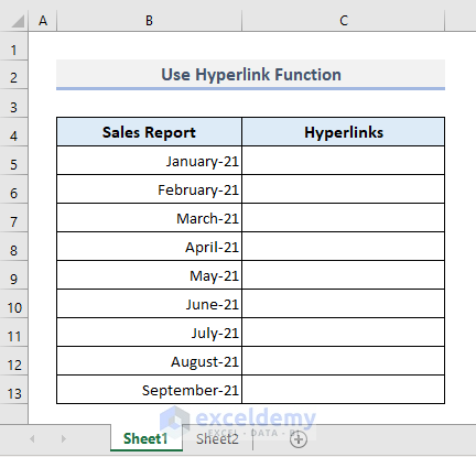

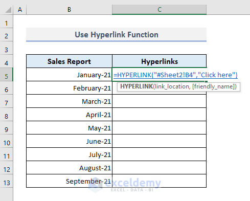
• Use the formula:

B4 in Sheet2 is referred to. The customized message is ‘Click here’.

• Press Enter to see the text with the hyperlink.

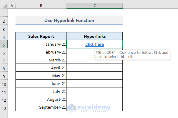
• Click the hyperlinked text in C5 in Sheet1 and you’ll be redirected to B4 in Sheet2.

Read More: How to Add Hyperlink to Another Sheet in Excel

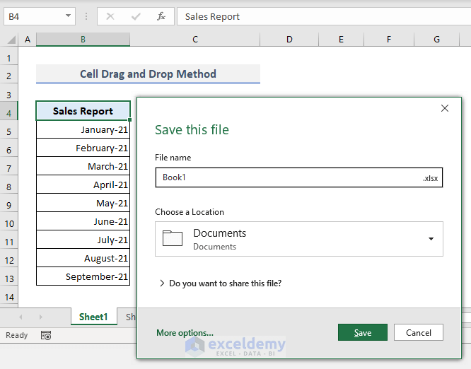
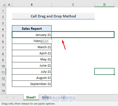
Method 3 – Applying the Cell Drag-and-Drop Method to Create a Hyperlink to Another Sheet

Save your workbook first.

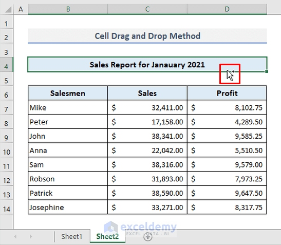
Step 1:

•  Drag your mouse pointer to the cell border of the reference value.

A Plus (+) sign will be displayed.

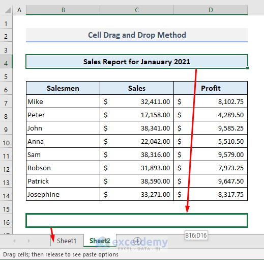
Step 2:

• Right-click.
• Hold the button and drag it in the Sheet name in which you want to add the hyperlink.
• Press and hold ALT.

Step 3:

• In the new worksheet, release ALT.
• Drag your mouse pointer to the cell in which you’ll add the hyperlink.
• Release the mouse pointer there and the Context Menu will open.

Step 4:

• Choose ‘Create Hyperlink Here’.

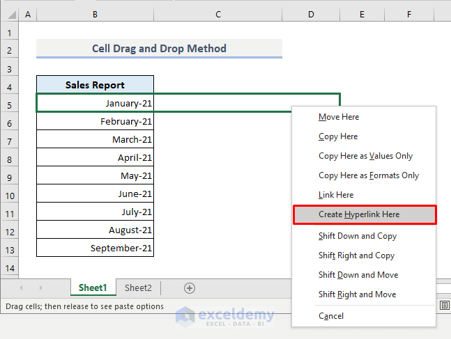
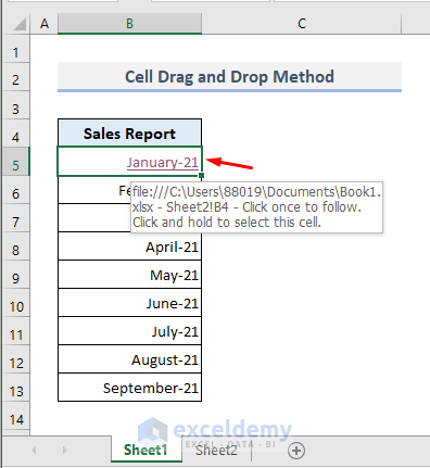
You’ll see the hyperlink.

Read More: How to Create a Drop Down List Hyperlink to Another Sheet in Excel

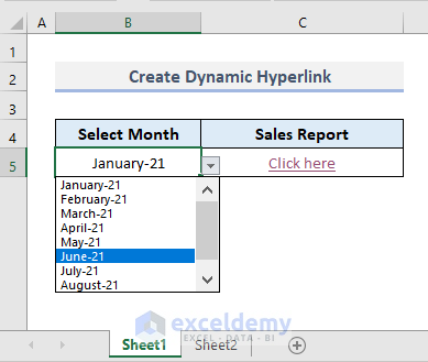
Method 4 – Create a Dynamic Hyperlink Based on the Cell Value with a Combined Formula

Create hyperlinks based on the values of a drop-down list.

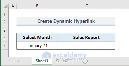
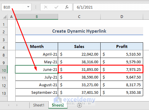
The image below is (Sheet2).

• Enter the formula in C5:

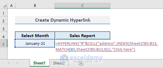
• Press Enter.

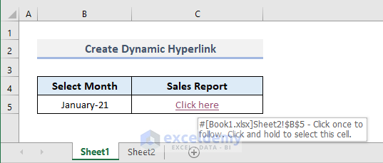
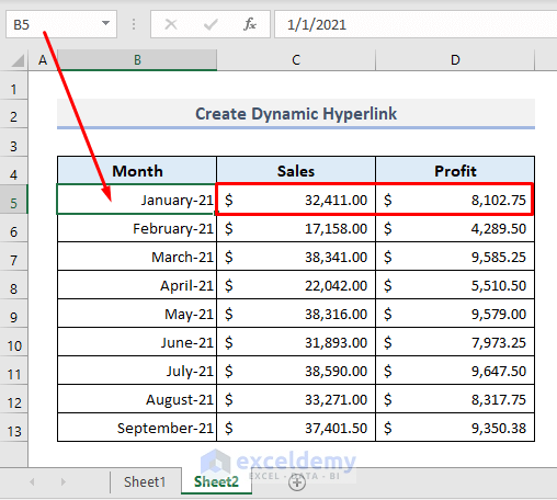
• Click the hyperlink in C5 and you’ll be redirected to B5 in Sheet2.

• You can select any other month (here, June-21) from the drop-down list in Sheet1.

• And click the hyperlink in C5.

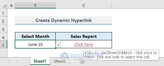
You’ll be now redirected to B10 in Sheet2.

Read More: How to Create Dynamic Hyperlink in Excel

Download Practice Workbook

Download the Excel workbook here.

You May Also Like to Explore

• How to Hyperlink to Cell in Same Sheet in Excel
• Excel Hyperlink to Cell in Another Sheet with VLOOKUP
• How to Combine Text and Hyperlink in Excel Cell
• How to Edit Hyperlink in Excel
• How to Copy Hyperlink in Excel
• How to Convert Text to Hyperlink in Excel
• How to Create Button to Link to Another Sheet in Excel

<< Go Back To Excel Hyperlink to Another Sheet | Hyperlink in Excel | Linking in Excel | Learn Excel