How to Convert Text to Hyperlink in Excel (5 Methods)

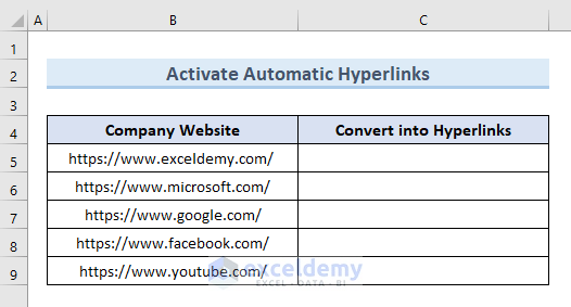
Method 1 – Activate Automatic Hyperlinks Option to Convert Text to Hyperlink in Excel

In the following dataset, we can see the URLs of 5 companies.

Steps:

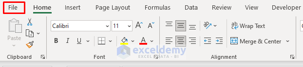
• Go to the File tab.

• Select Options.

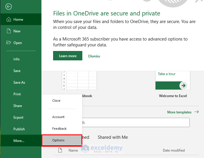
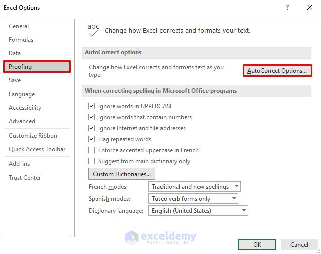
• A new dialog box for Excel Options will appear.
• Go to the Proofing section and select AutoCorrect Options.

• A box named AutoCorrect will appear.
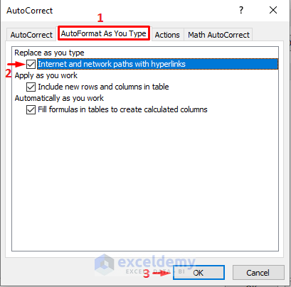
• Select AutoFormat As You Type.
• Check the option Internet and network paths with hyperlinks.
• Click on OK.

• Close all dialog boxes.
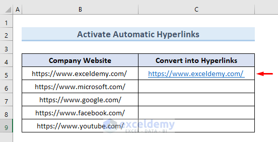
• When you input the first URL manually in cell C5 and press Enter, it will automatically get converted into a hyperlink.

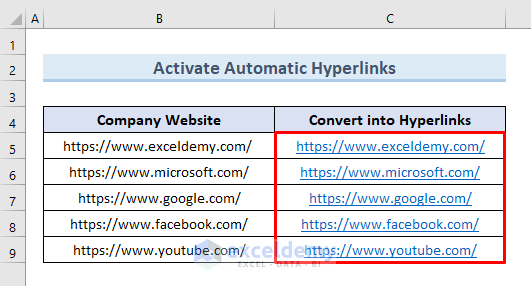
• We manually copied over all URLs and they got converted.

Read More: How to Combine Text and Hyperlink in Excel Cell

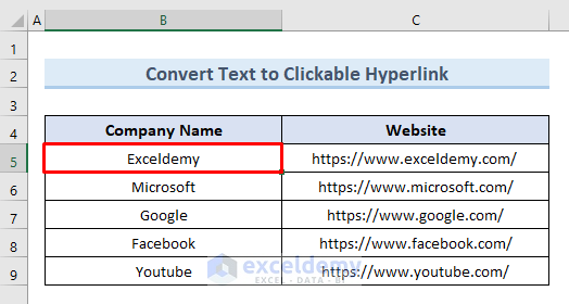
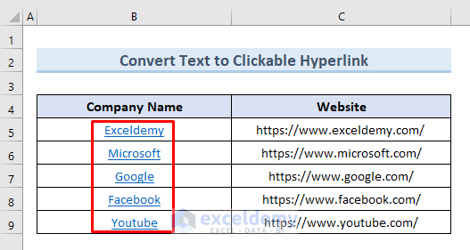
Method 2 – Convert Text of a Cell into a Clickable Hyperlink Using the Excel Ribbon

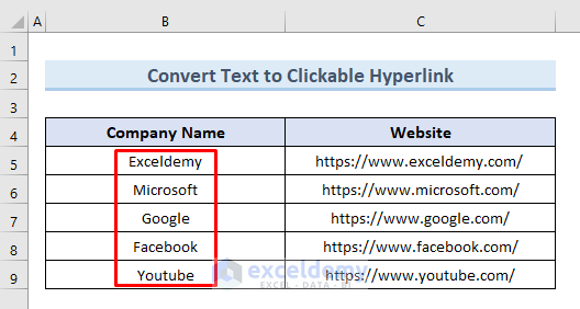
We have names of companies and their website URLs. We will convert the names of companies into clickable hyperlinks.

Steps:

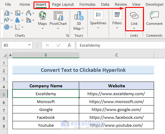
• Select cell B5.

• Go to the Insert tab from the ribbon and select the option Link.

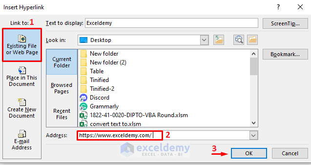
• A new dialog box will appear.
• Select the option Existing File or Web Page.
• Insert the link to that company in the Address.
• Click on OK.

• We get a clickable link in the company name Exceldemy. If we click on the company name, it will take us to the website.

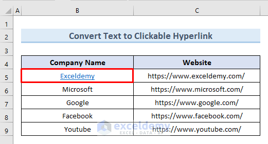
• Repeat to convert all the company names into clickable links.

Read More: How to Hyperlink to Cell in Excel

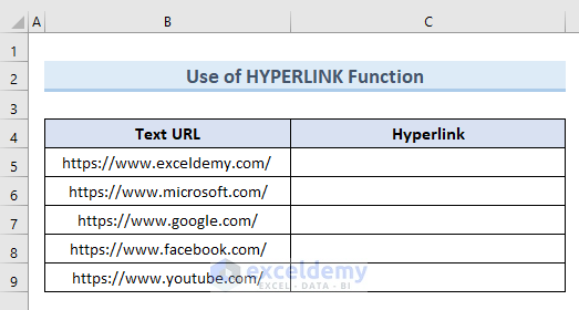
Method 3 – Apply the HYPERLINK Function to Convert Text to Hyperlink

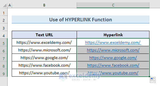
We have the following dataset of URLs of 5 companies in column B. We will create hyperlinks for these URLs in column C.

Steps:

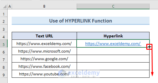
• Select cell C5 and insert the following formula:

• Press Enter.

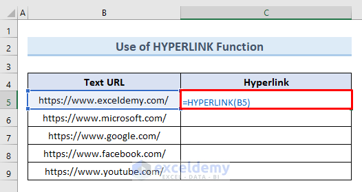
• This creates a hyperlink for the URL in cell B5.

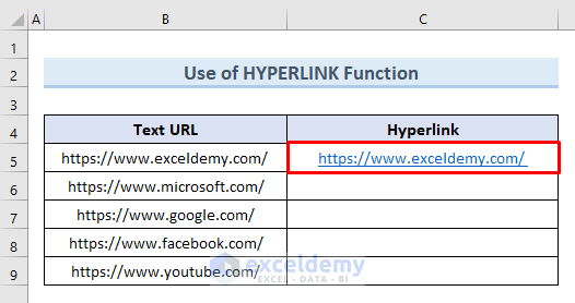
• Drag the Fill Handle tool to the end of the data range.

• In column C, we get hyperlinks for all the URLs from column B.

Read More: How to Edit Hyperlink in Excel

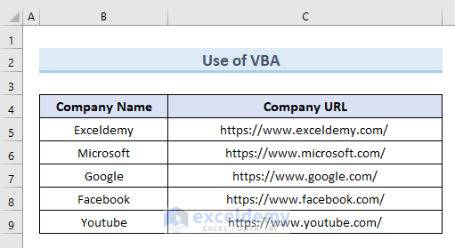
Method 4 – Use VBA Code to Convert Text to Hyperlink in Excel

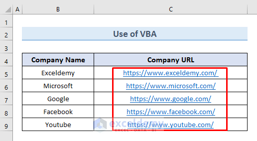
We will convert the URLs of companies into hyperlinks.

Steps:

• Go to the Developer tab and select the Visual Basic option from the ribbon.

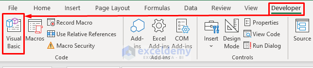
• This will open the Bisual Basic window.
• Go to the Insert tab and select Module.

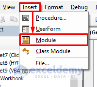
• A new blank VBA Module will appear.
• Insert the following code in that module:

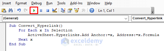
Sub Convert_Hyperlink()
For Each x In Selection
ActiveSheet.Hyperlinks.Add Anchor:=x, Address:=x.Formula
Next x
End Sub

• Click on Run or press the F5 key to run the code.

• All the URLs of column C are now converted into hyperlinks.

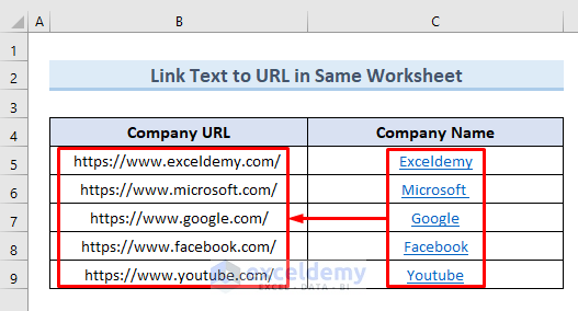
Method 5 – Convert Text to Hyperlink to Link in Same Worksheet

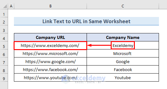
We will link one cell with another cell in the same worksheet whereas in the previous examples we linked a URL with a text value in a particular cell. For example, we will link cell C5 with cell B5, so clicking on the hyperlink of cell C5 will take us to cell B5.

Steps:

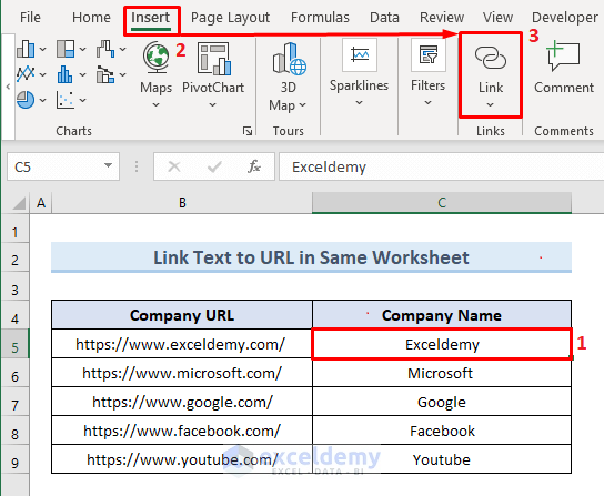
• Select cell C5.
• Go to the Insert tab and select the option Link.

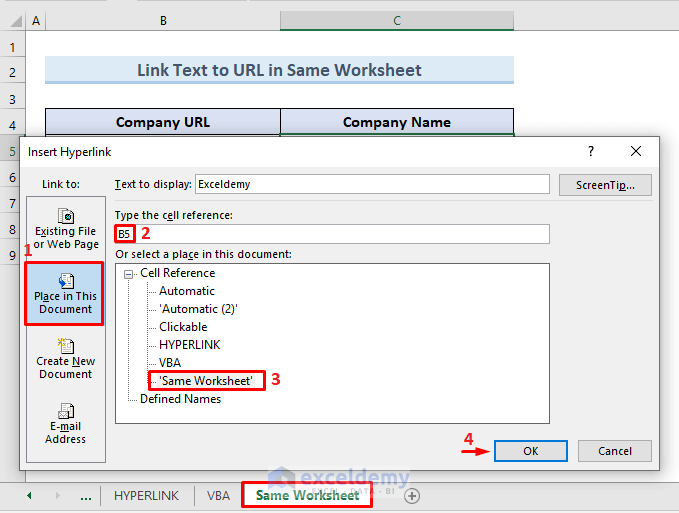
• A new dialog box named Insert Hyperlink will appear.
• From the Link to section, select the option Place in this Document.
• Input the value B5 in the section named Type the cell reference. This links the cell C5 with cell B5.
• Select the option Same Worksheet to identify the place of this document.
• Click on OK.

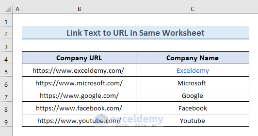
• We can see the company name Exceldemy is now converted into a hyperlink.

• If we click on the hyperlink of cell C5, it will take us to cell B5.

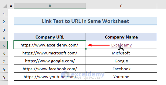
• We can repeat the process for all the cells.

Read More: How to Hyperlink to Cell in Same Sheet in Excel

Download the Practice Workbook

Related Articles

• Excel Hyperlink to Cell in Another Sheet with VLOOKUP
• How to Add Hyperlink to Another Sheet in Excel
• Excel Hyperlink to Another Sheet Based on Cell Value
• How to Create a Drop Down List Hyperlink to Another Sheet in Excel
• How to Create Dynamic Hyperlink in Excel
• How to Copy Hyperlink in Excel
• How to Create Button to Link to Another Sheet in Excel

<< Go Back To Hyperlink in Excel | Linking in Excel | Learn Excel