How to Use SUMIFS When Cells Are Not Equal to Multiple Text

We can use conditional summation using the SUMIF and SUMIFS functions in Excel. The SUMIFS function is available from Excel version 2010. This function can accept multiple criteria and multiple sum ranges. In this article, we will show you 3 easy methods to use SUMIFS when cells are not equal to multiple texts in Excel.

SUMIFS Not Equal to Multiple Text: 3 Handy Approaches

We will show you three quick and easy ways to use SUMIFS when cells are not equal to multiple texts. For the first method, we will simply use the SUMIFS function. Then, we will subtract the SUMIFS amount from the whole total calculated using the SUM function. Lastly, we will combine SUM and SUMIFS functions to achieve our goal.
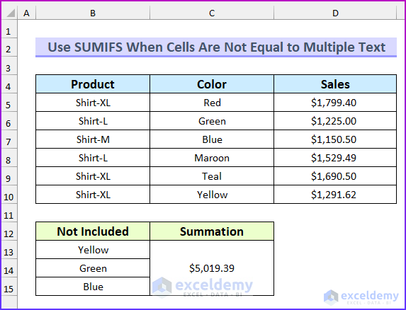
To demonstrate the methods, we have selected a dataset that has three columns consisting of “Product”, “Color”, and “Sales”. Then, we will find the sales for the products that are not yellow, green, or blue.

1. Applying SUMIFS Function

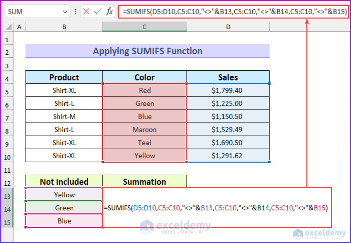
In this first method, we will use the SUMIFS function to get the sales total for the colors red, teal, and maroon. That means the not equal to multiple text part is equal to the colors yellow, green, and blue. We will exclude these when we calculate the sales total.

Steps:

To begin with, type the following formula in cell C13. Here, we have merged the cells C13:C15.

=SUMIFS(D5:D10,C5:C10,"<>"&B13,C5:C10,"<>"&B14,C5:C10,"<>"&B15)

Next, press ENTER.
So, this will return the total value excluding those three colors.

Formula Breakdown

Firstly, the sum range is D5:D10.
Secondly, there are three same criteria range C5:C10.
Thirdly, we are excluding the colors using the not equal “<>” operator and joining those with the cell values using the ampersand (“&”).

2. Subtracting SUMIFS from SUM Function

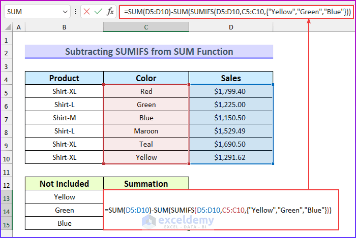
We will calculate the overall sales total using the SUM function in this method. Then, we will find the summation of the sales for the three colors: yellow, green, and blue. Lastly, we will subtract this value from the previous value to reach the goal of this article.

Steps:

Firstly, type the following formula in cell C13. Here, we have merged the cells C13:C15.

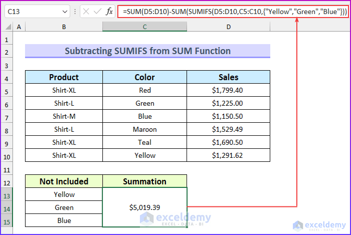
=SUM(D5:D10)-SUM(SUMIFS(D5:D10,C5:C10,{"Yellow","Green","Blue"}))

Next, press ENTER.
Hence, this will return the total value excluding those three colors.

Formula Breakdown

SUM(D5:D10)
- Output: 8686.51.
SUMIFS(D5:D10,C5:C10,{“Yellow”,”Green”,”Blue”})
- Output: {1291.62,1225,1150.5}.
- The sum range is D5:D10. Then, the criteria range is C5:C10. This only finds the sales value for those three colors.
Then, the formula becomes → 8686.51-SUM({1291.62,1225,1150.5})
- Output: 5019.39.
- Lastly, we subtract the values to get the sales total for the other three colors.

3. Combining SUM and SUMIFS Function

We will combine the SUM and SUMIFS functions in this last method to use SUMIFS when cells are not equal to multiple texts in Excel.

Steps:

To begin with, type the following formula in cell C13. Here, we have merged the cells C13:C15.

=SUM(SUMIFS(D5:D10,C5:C10,{"*","Yellow","Green","Blue"})*{1,-1,-1,-1})

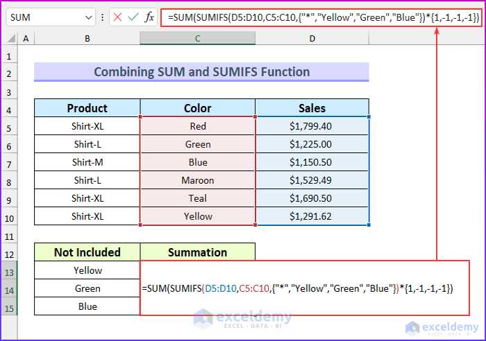
Then, press ENTER.
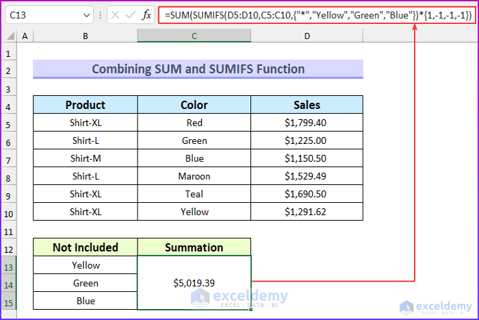
So, this will return the total value excluding those three colors.

Formula Breakdown

Firstly, the portion inside the SUM function is → SUMIFS(D5:D10,C5:C10,{“*”,”Yellow”,”Green”,”Blue”})*{1,-1,-1,-1}
- Output: {8686.51,-1291.62,-1225,-1150.5}.
- Here the sum range is D5:D10 and the criteria range is C5:C10.
- Then, there are four parts of the criteria. We have included the asterisk (“*”) to include all the sales.
- After that, we used another array to multiply the values. The positive sign is for the total sales amount and the negative sign is for the three excluded colors.
Then, the formula reduces to → SUM({8686.51,-1291.62,-1225,-1150.5})
- Output: 5019.39.
- Finally, we sum the values to get the result.

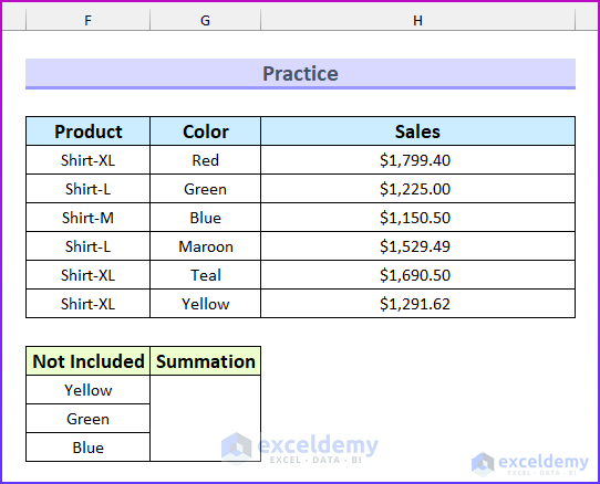
Practice Section

We have added a practice dataset for each method in the Excel file. Therefore, you can follow along with our methods easily.

Download Practice Workbook

You can download the Excel file from the link below.

Applying SUMIFS Not Equal to Multiple Text.xlsx

Conclusion

We have shown you three quick methods to use SUMIFS when cells are not equal to multiple texts in Excel. If you face any problems regarding these methods or have any feedback for me, feel free to comment below. However, remember that our website implements comment moderation. Therefore, your comment may not be instantly visible. So, have a little bit of patience, and we will solve your query as soon as possible.