Mortgage Calculator with Extra Payments and Lump Sum in Excel

Using A Mortgage/Loan Calculator with Extra Payments & Lump Sum in Excel

This calculator can be used to:

Calculate your regular payments (PMT).
Deposit recurring extra payments.
Deposit irregular / lump-sum payments.

The template will showcase the following outputs:

The total amount paid over the lifetime of the loan
Total interest paid
Estimated interest savings (if you made recurring extra payments or irregular/lump sum extra payments)
Total number of payments
Time saved (if you made recurring extra payments or irregular/lump sum extra payments)

Further options:

Two types of payment
- End of the Period
- Beginning of the Period
Interest Compounding Frequency.
A different payment frequency for your extra recurring payments.

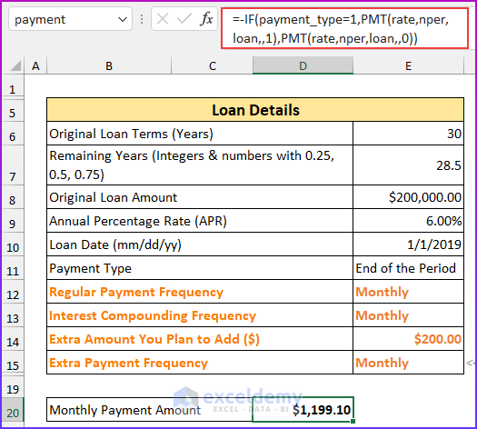
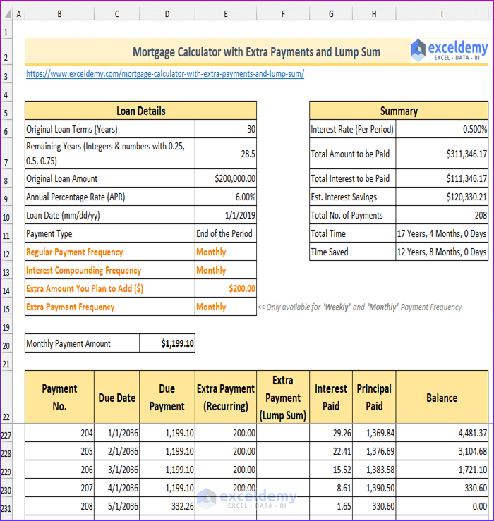
Consider the following example:

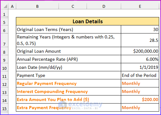
Original Loan Amount: $200,000
Original Loan Terms (Years): 30
Remaining Years: 28.50
Annual Percentage Rate: 6%
Loan Date (mm/dd/yy): 1/1/2019
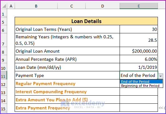
Payment Type: End of the Period
Regular Payment Frequency: every month.
Interest Compounding Frequency: Monthly. This is the normal case: the Regular Payment Frequency is the same as the Interest Compounding Frequency. For different Interest Compounding Frequency & Regular Payment Frequency, Interest Compounding Frequency must be equal to or higher than the frequency of the Regular Payment.
Extra Amount You Plan to Add ($): 200.
Extra Payment Frequency: $200 every month. You can also choose Bi-monthly, Quarterly, Semi-annually, Annually. For “Monthly” Extra Payment Frequency, you cannot choose Weekly or Bi-weekly frequencies. The template will show errors.
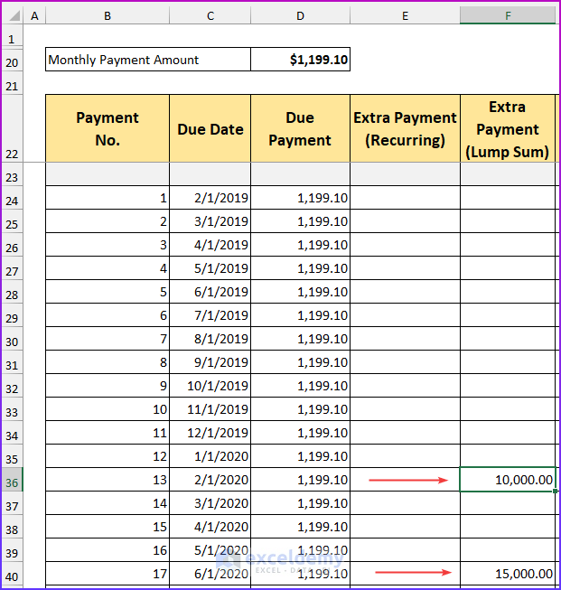
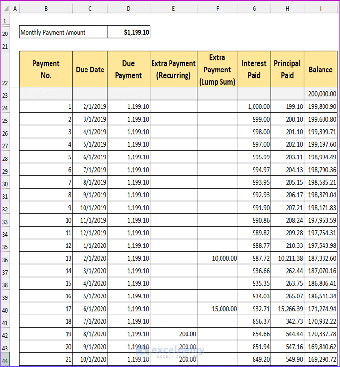
Adding Lump Sum Payments: On the 13^th and 17^th periods, let’s add two lump sum payments, $10,000 and $15,000. You will enter these values directly in the column Extra Payment (Lump Sum).

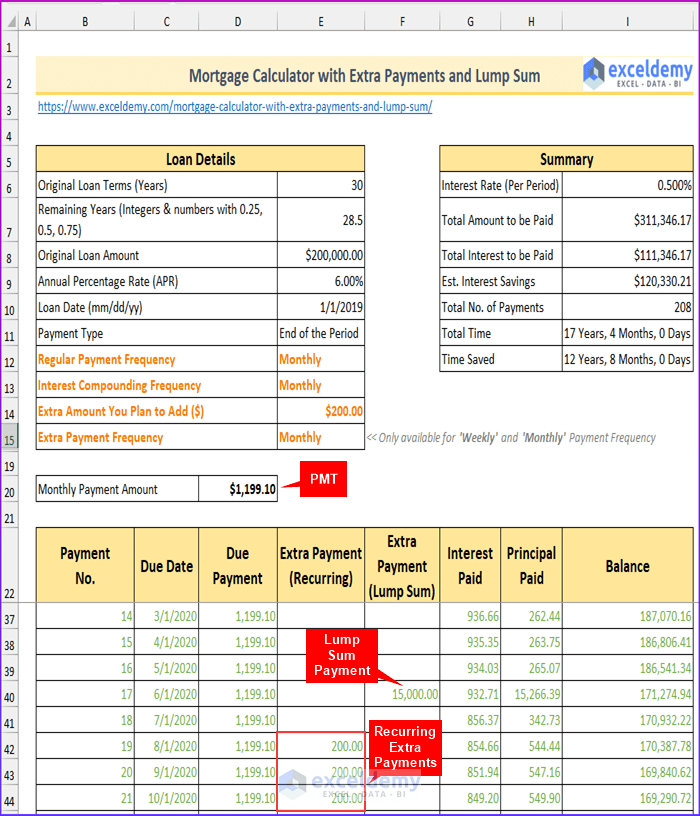
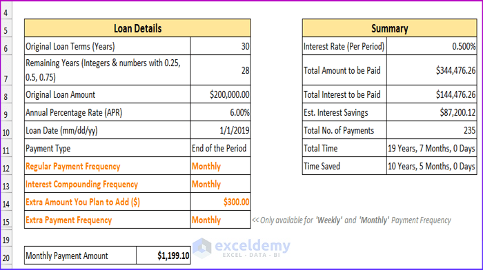
Here is the loan summary:

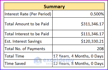
We are saving:

Interest: $120,330.21
Time: 12 years and 8 months

Mortgage Calculator with Extra Payments and Lump Sum in Excel – Easy Steps

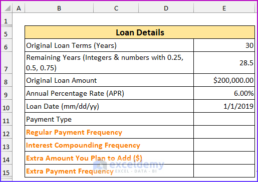
Step 1: Entering Loan Details

To enter the loan details, use the Name Range and Data Validation features of Excel and apply the IF, PMT, and VLOOKUP functions.

Enter the values. Here, 28.5 in the remaining years field.

Press ALT, M, and N (one after the other) to see the Name Manager dialog box.

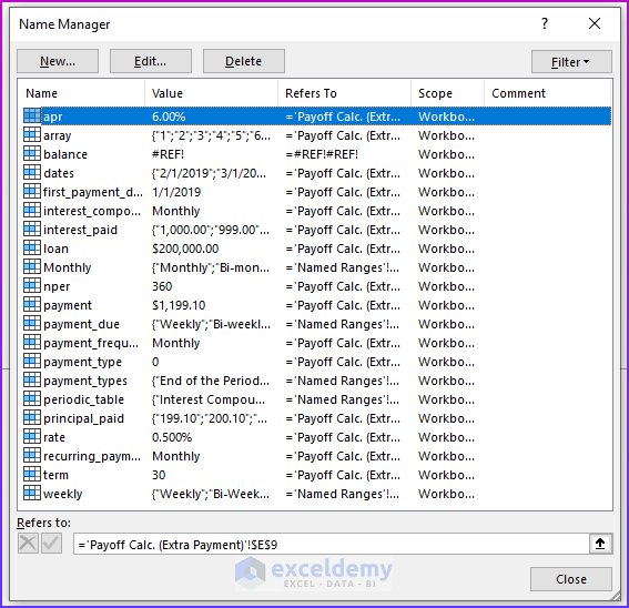
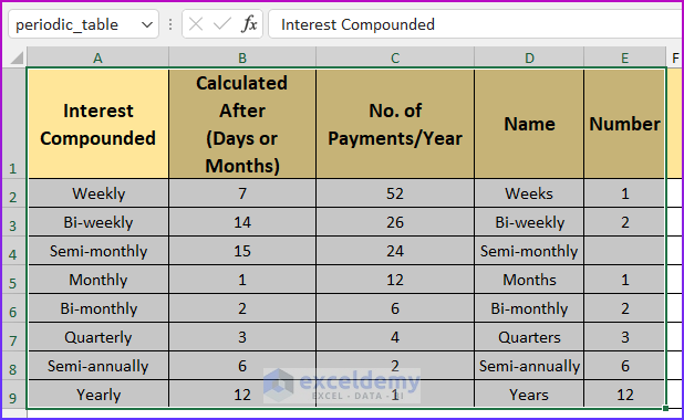
The “periodic_table” is in a hidden sheet to avoid accidentally changing the values.

Select E11 and press ALT, A, V, and then V (one after the other) to open the data validation dialog box.
In Allow:, select List.
In Source, enter =payment_types.
Click OK.

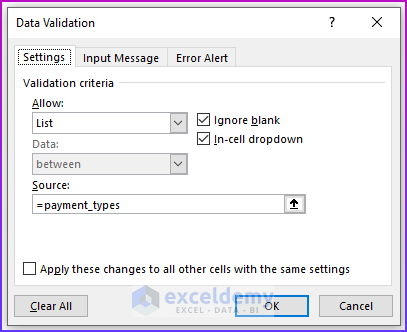
Two items will be displayed in the dropdown list.

Repeat the above steps for E12, E13, and E15. Source will be “=payment_due” for E12 and E13. For E15 it will be “=INDIRECT(payment_frequency)”. Remember, the extra payment frequency is only available for “weekly” and “monthly” payment frequencies.
Enter the number of extra payments in E14. Here, $200.

Enter this formula to find the value of the installment amount. The PMT function is used, here.

=-IF(payment_type=1,PMT(rate,nper,loan,,1),PMT(rate,nper,loan,,0))

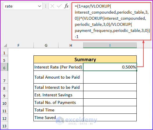
Enter the following formula to calculate the interest rate per period.

=(1+apr/VLOOKUP(interest_compounded,periodic_table,3,0))^(VLOOKUP(interest_compounded,periodic_table,3,0)/VLOOKUP(payment_frequency,periodic_table,3,0))-1

Formula Breakdown

The three VLOOKUP functions return a value from the third column and match it with the lookup range.
VLOOKUP(interest_compounded,periodic_table,3,0)
- Output: 12.
VLOOKUP(payment_frequency,periodic_table,3,0)
- Output: 12.
The formula reduces to, (1+apr/12)^(12/12)-1
- Output: 0.00499999999999989.

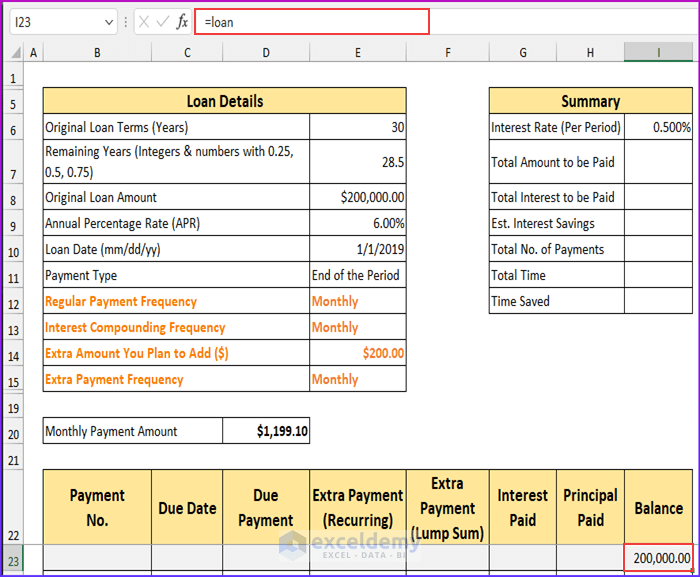
Step 2: Calculating the Payment Schedule

To calculate the mortgage payment schedule with extra payments and a lump sum, the IFERROR, AND, OR, EDATE, and MOD functions will be used.

Create the row headings as shown in row 22.
Enter the following formula to see the beginning balance.

=loan

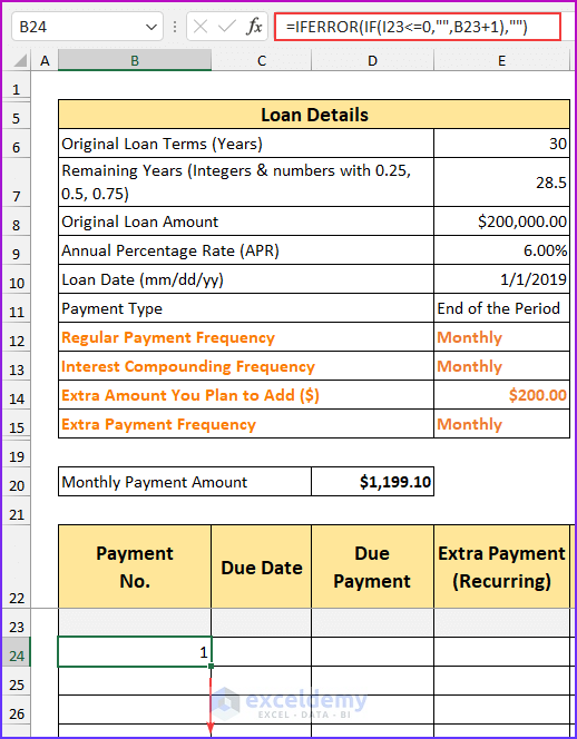
Enter this formula to see the payment number, and use the Fill Handle to copy the formula.

=IFERROR(IF(I23<=0,"",B23+1),"")

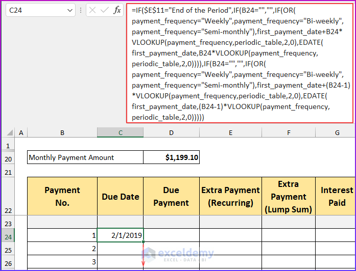
Enter this formula to see the due date and use the Fill Handle to copy the formula.

=IF($E$11="End of the Period",IF(B24="","",IF(OR(payment_frequency="Weekly",payment_frequency="Bi-weekly",payment_frequency="Semi-monthly"),first_payment_date+B24*VLOOKUP(payment_frequency,periodic_table,2,0),EDATE(first_payment_date,B24*VLOOKUP(payment_frequency,periodic_table,2,0)))),IF(B24="","",IF(OR(payment_frequency="Weekly",payment_frequency="Bi-weekly",payment_frequency="Semi-monthly"),first_payment_date+(B24-1)*VLOOKUP(payment_frequency,periodic_table,2,0),EDATE(first_payment_date,(B24-1)*VLOOKUP(payment_frequency,periodic_table,2,0)))))

Formula Breakdown

OR(payment_frequency=”Weekly”,payment_frequency=”Bi-weekly”,payment_frequency=”Semi-monthly”)
- Output: FALSE.
first_payment_date+B24*VLOOKUP(payment_frequency,periodic_table,2,0)
- Output: 43467.
EDATE(first_payment_date,B24*VLOOKUP(payment_frequency,periodic_table,2,0))
- Output: 43497.
first_payment_date+(B24-1)*VLOOKUP(payment_frequency,periodic_table,2,0)
- Output: 43466.
EDATE(first_payment_date,(B24-1)*VLOOKUP(payment_frequency,periodic_table,2,0))
- Output: 43466.
The formula reduces to, IF($E$11=”End of the Period”,IF(B24=””,””,IF(FALSE,43467,43497)),IF(B24=””,””,IF(FALSE,43466,43466)))
- Output: 43497.
- February 01, 2019.

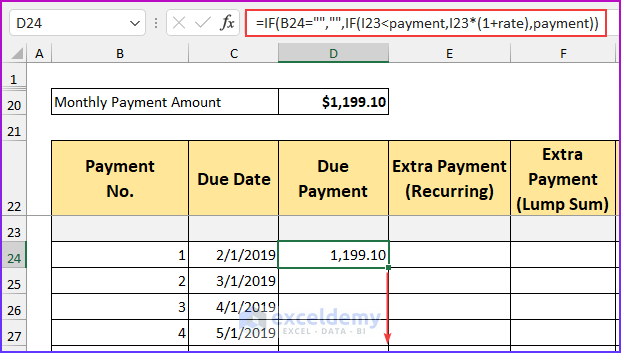
Enter this formula to see the due payment and drag the Fill Handle to copy it.

=IF(B24="","",IF(I23<payment,I23*(1+rate),payment))

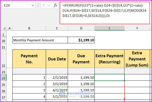
Enter this formula for the recurring extra payments.

=IFERROR(IF(I23*(1+rate)-D24<$E$14,I23*(1+rate)-D24,IF(B24=$I$17,$E$14,IF(B24<$I$17,0,IF(MOD(B24-$I$17,$E$18)=0,$E$14,0)))),0)

Formula Breakdown

IF(B24=$I$17,$E$14,IF(B24<$I$17,0,IF(MOD(B24-$I$17,$E$18)=0,$E$14,0)))
- Output: 0.
I23*(1+rate)-D24
- Output: 199800.898949694.
I23*(1+rate)-D24<$E$14
- Output: FALSE.
The formula reduces to, IFERROR(IF(FALSE,199800.898949694,0),0)
- Output: 0.
- As the condition of IF is false, it will return the value of zero.

Enter the lump sum amount manually.

Enter this formula and drag down the Fill handle to copy it. The interest paid amount will be displayed.

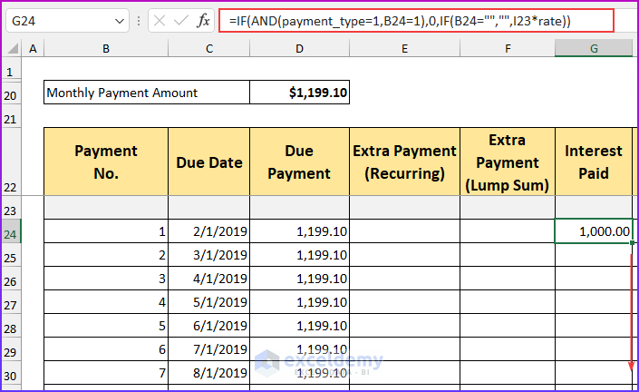
=IF(AND(payment_type=1,B24=1),0,IF(B24="","",I23*rate))

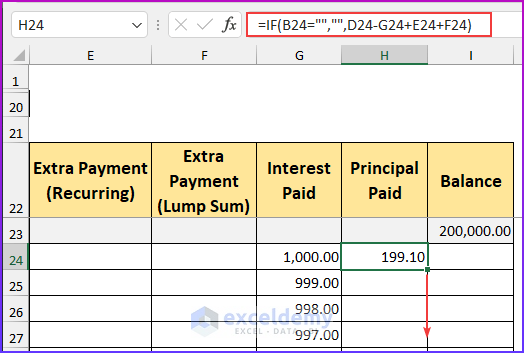
Enter this formula to see the principal amount.

=IF(B24="","",D24-G24+E24+F24)

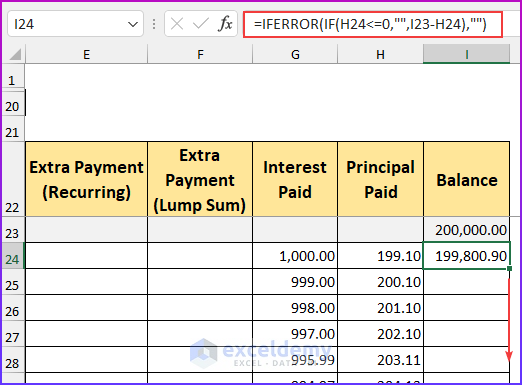
Enter this formula to see the ending balance amount.

=IFERROR(IF(H24<=0,"",I23-H24),"")

This is the final output.

Step 3: Finding the Summary Amount

The SUM, COUNTIF, DATEDIF, INDEX, and OFFSET functions will be used.

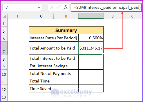
Enter this formula to see the total amount to be paid.

=SUM(interest_paid,principal_paid)

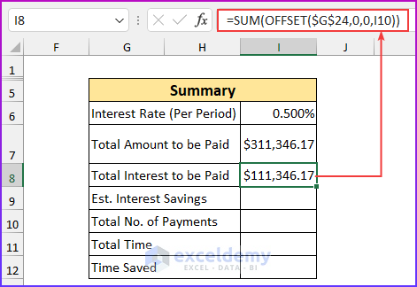
Enter this formula to see the total amount of interest to be paid.

=SUM(OFFSET($G$24,0,0,I10))

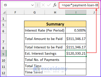
Enter the following formula to see the value of the estimated interest savings.

=nper*payment-loan-I8

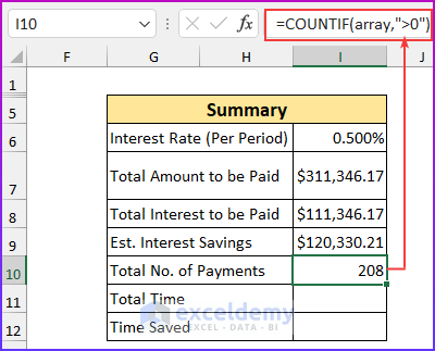
Enter this formula to see the total number of payments.

=COUNTIF(array,">0")

Enter the following formula to calculate the total time.

=DATEDIF(first_payment_date,INDEX(dates,I10),"y") & " Years, " & DATEDIF(first_payment_date,INDEX(dates,I10),"ym") & " Months, " & DATEDIF(first_payment_date,INDEX(dates,I10),"md") & " Days"

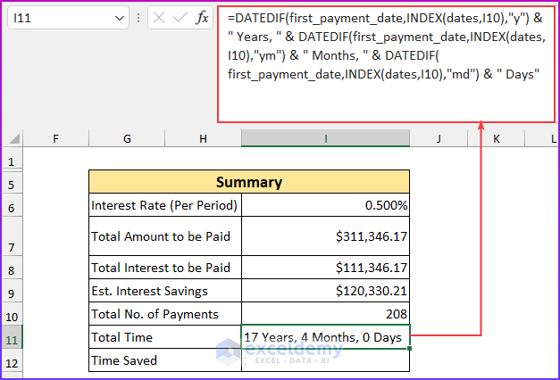
Formula Breakdown

INDEX(dates,I10)
- Output: 49796.
DATEDIF(first_payment_date,49796,”y”)
- Output: 17.
- Here, “y” was used to return the number of years. By entering “ym” and “md” the function will return month and day.
The formula reduces to, =17 & ” Years, ” & 4 & ” Months, ” & 0 & ” Days”
- Output: 17 Years, 4 Months, 0 Days.

Enter this formula to return the value of the time saved.

=DATEDIF(INDEX(dates,I10),EDATE(first_payment_date,term*12),"y") & " Years, " & DATEDIF(INDEX(dates,I10),EDATE(first_payment_date,term*12),"ym") & " Months, " & DATEDIF(INDEX(dates,I10),EDATE(first_payment_date,term*12),"md") & " Days"

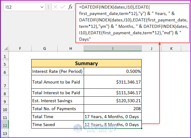
This is the final mortgage calculator with extra payments and the lump sum in Excel.

Cautions:

1) If the interest compounding frequency is lower than the frequency of regular payment, the template will show an error.

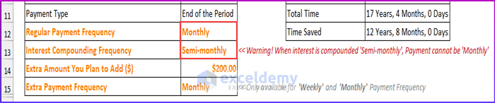
You see an error showing when the interest compounding frequency is Semi-monthly and the regular payment frequency is monthly:

<< Warning! When interest is compounded ‘Semi-monthly’, payment cannot be ‘Monthly’

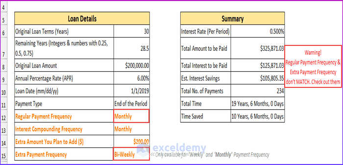
2) The Extra Payment Frequency will be equal to or greater than the Regular Payment Frequency.

Observe the image below. Our regular payment frequency is monthly, but our extra payment frequency is Bi-Weekly. The error message is displayed.

“Warning! Regular Payment Frequency & Extra Payment Frequency don’t MATCH. Check out them”

Mortgage Interest Is Tax-Free. Is It Wise to be Debt Free?

In The USA mortgage interests are tax-free.

Consider the following example: You’re planning to pay $1200 every month for your $200,000 loan at a 6% APR for the next 30 years. You earn $4000 a month, and you’re in the 25% tax bracket. For the next 30 years, you save $300 in tax every month on your $4000 income. The total savings is $108,000.

How to Calculate an Early Paying Off Your Debt:

After 2 years, you pay $300 every month. So, you save $75 every month in tax exemptions. Total tax savings = $75 x 19 years, 7 months = $17,625 Total tax exemptions for regular monthly payments: $300 x 19 years, 7 months = $70,500

The loan is paid in 19 years and 7 months. Your total savings will be: ($1200 – $300) x 10 years 5 months = $112,500. $300 in tax savings were deducted from your monthly payment of $1200. Grand savings total will be: $17,625 + $70,500 + $112,500 = $200,625

Things to Consider Before Paying Off Your Loan Earlier

Are there any prepayment penalties?
Do you have any high-paying credit cards or any other debts? Pay them first. Mortgage loan interest rates are the lowest in the debt world.

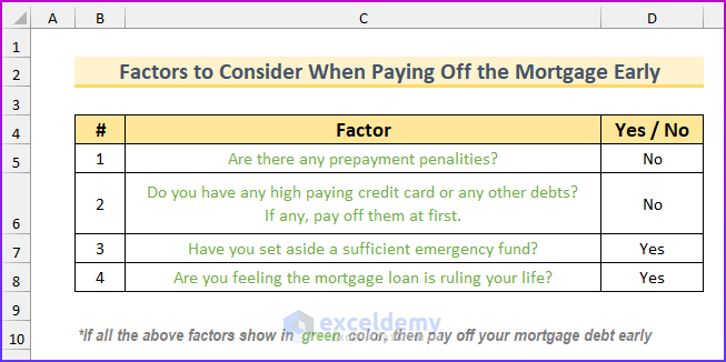
There’s a prepayment checklist in the template workbook.

Auto Loan Calculator with Extra Payments and Lump Sum

The existing template can be used as an auto loan calculator with extra payments and a lump sum.

Download Practice Workbook

Download the Excel file here.

Creating Mortgage Calculator with Lump Sum.xlsx

<< Go Back to Mortgage Calculator | Finance Template | Excel Templates

Get FREE Advanced Excel Exercises with Solutions!

14 Comments

Jaime Franco Jun 4, 2019 at 10:28 PM

Hey, This calculator is great! The only thing I added, and I think would probably be a help to people, is some summaries for what has already been spent towards principal and interest, and what is remaining on both.
- Reply
  Kawser Jun 8, 2019 at 2:20 PM
  
  I am keeping your note. Thanks, Jaime for your feedback.
  Best regards
  Kawser Ahmed
  - Reply
    karen ling Dec 10, 2021 at 6:25 PM
    
    Hi Kawser,
    
    the excelsheet is great but if there is variable interest along the tenure and variable extra payment which can help to reduce tenure period.
    - Rafi Sep 4, 2022 at 4:51 PM
      
      Hi KAREN LING,
      Glad that you liked the template. This template has got fixed interest rate. You can add variable extra payments manually to your Excel file if you need it.
      Regards,
      Rafi (ExcelDemy Team)
Mike Feb 26, 2021 at 11:51 PM

Hi, Thanks for the template. I live in the U.K. and, for many mortgages, interest is charged daily, so any overpayments reduce the interest amount straight away. Consequently it would be useful to be able to add the actual dates and amounts for the overpayments (rather than just the current month ‘period’ possible at the moment).
Incidentally, the first payment is usually taken on a different date to the subsequent monthly payments (so the first payment is slightly different to take this different payment date into account).
Any improvements to the template to include these would be great 🙂 Thanks!
- Reply
  Kawser Mar 4, 2021 at 12:08 AM
  
  Hi Mike,
  I am taking note of your problem, we shall make templates on the basis of your needs.
  Thanks.
Jon May 11, 2022 at 9:26 PM

Really good calculator, however I pay a regular amount and the is reduces the minimum payment not the the term. Example I always make monthly payment of 1000 however the minimum payment is 750 for month 1, then 749 for month 2 etc. Is this possible?
- Reply
  Rafi Sep 4, 2022 at 4:32 PM
  
  Hi JON,
  Thanks for your feedback. Can you please elaborate on your problem?
  What I can say is that paying an extra amount from the minimum will reduce the next payments. You can proceed with your data. You can also share your Excel file with us and we will look into it.
  Regards.
  Rafi (ExcelDemy Team)
Violet Dec 31, 2022 at 7:22 AM

Does the PMT include taxes and insurance? For example, I have a PMT of $1308 that includes my taxes/insurance. Without it, the PMT is around $1100. Which number do I put in the spreadsheet as the PMT?
- Reply
  Guria Jan 1, 2023 at 5:26 PM
  
  Hello Violet,
  Thanks for sharing your query. Yes, the PMT does include tax or insurance. Therefore, you will provide $1308 as the PMT in your spreadsheet.
  Let us know if you have more queries.
  
  Regards,
  Guria
  ExcelDemy.
Nicola Jan 27, 2023 at 4:38 PM

Thanks for this spreadsheet. Can you please explain how I adjust the rate increases when the bank does. ie for the first 6 month I was on 7.5% interest per annum and now it is 8% Sorry, I am not very good with excel that is why I am using your preformulated one! Many thanks.
- Reply
  Guria Jan 31, 2023 at 5:28 PM
  
  Hello Nicola,
  Thank you for sharing your problem. I assume you are getting difficulties to calculate interest rate as changed twice in a year. In that case, calculate first 6 months’ rate separately with this formula =7.5/12 and later 6 months’ with =8/12. As a result, you will get the values of monthly interests.
  I hope this solution will help you. Let us know your feedback.
  
  Regards,
  Guria
  ExcelDemy
Mohammed Jul 26, 2023 at 3:46 AM

Hi all, this calculator is GREAT! thank you. The only column missing is Early Repayment Charge (ERC) which changes through out the Fixed term is (5% in 1st year; 4% in the second; 3.5% in the third… etc)

I have tried adding the column ‘J’ manually and inserting the following formulas next to each line for months 2-11 (skipping the first month in each year for the 10% early repayment allowance) in this example J25=F25/100*5; J37=F37/100*4; J49=F49/100*3.5) which works fine for calculating the ERC value. However, it does not take into account that the remaining balance (column ‘I’ on which the interest and capital repayment calculations are based on) have in fact increased by the amount of the ERC column ‘J’ value calculated in the previous line.

I have worked it out by adding the value from previous line in ‘J’ column to the end of the formula in ‘I’ column:
I25 =IFERROR(IF(H25<=0,"",I24-H25),"")+J24
I26 =IFERROR(IF(H26<=0,"",I25-H26),"")+J25 etc…

The calculations seems to be correct. I wonder if there is any better way of achieving similar result?
- Reply
  Akib Bin Rashid Jul 26, 2023 at 12:56 PM
  
  Hi Mohammed
  Thank you for your appreciation. If you want to incorporate ERC in your final balance, I think your method is a nice one.
  I would, however, suggest one thing. Keep the ERC in column I and calculate the final balance in column J.

Mortgage Calculator with Extra Payments and Lump Sum in Excel – Easy Steps

Using A Mortgage/Loan Calculator with Extra Payments & Lump Sum in Excel

Mortgage Calculator with Extra Payments and Lump Sum in Excel – Easy Steps

Step 1: Entering Loan Details

Step 2: Calculating the Payment Schedule

Step 3: Finding the Summary Amount

Cautions:

Mortgage Interest Is Tax-Free. Is It Wise to be Debt Free?

Things to Consider Before Paying Off Your Loan Earlier

Auto Loan Calculator with Extra Payments and Lump Sum

Related Articles

Leave a reply Cancel reply