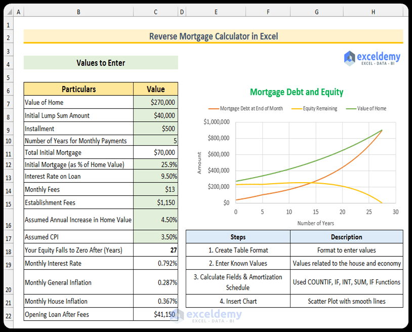
Here’s an overview of the calculator we’ll make.
How to Create a Reverse Mortgage Calculator in Excel (With Easy Steps)
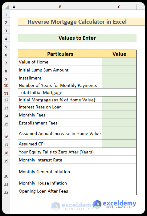
Step 1 – Create the Required Fields
The green fill indicates the cell values will be specified by the users. We will insert the formulas in the other cells.
- Create the following fields –
- Value of Home
- Initial Lump Sum Amount
- Installment
- Number of Years for Monthly Payments
- Total Initial Mortgage
- Initial Mortgage (as % of Home Value)
- Interest Rate on Loan
- Monthly Fees
- Establishment Fees
- Assumed Annual Increase in Home Value
- Assumed CPI – CPI means Consumer Price Index.
- Your Equity Falls to Zero After (Years)
- Monthly Interest Rate
- Monthly General Inflation
- Monthly House Inflation
- Opening Loan After Fees
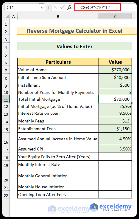
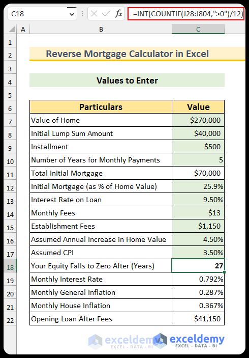
Step 2 – Enter Known Values
- Input the known values in the table.
- Use this formula in cell C11 to find the total initial mortgage.
=C8+C9*C10*12
- Insert this formula to find the monthly interest rate in cell C19.
=C13/12
- Use this formula in cell C20 to return the monthly general inflation.
=(1+C17)^(1/12)-1
- Insert the following formula which will calculate the monthly house inflation in cell C21.
=(1+C16)^(1/12)-1
- Use this formula in cell C22 to find the opening loan after including the establishment fees.
=C8+C15
- The value of cell C18 is missing, and we will find this value after completing the third step.
Read More: How to Create Fixed Rate Mortgage Calculator in Excel
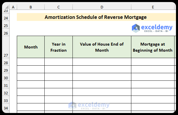
Step 3 – Create the Amortization Schedule
- Create the following headers:
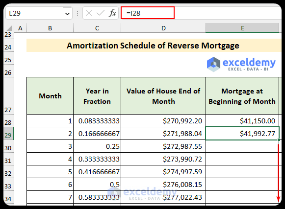
- Month
- Year in Fraction
- Value of House End of Month
- Mortgage at the Beginning of the Month
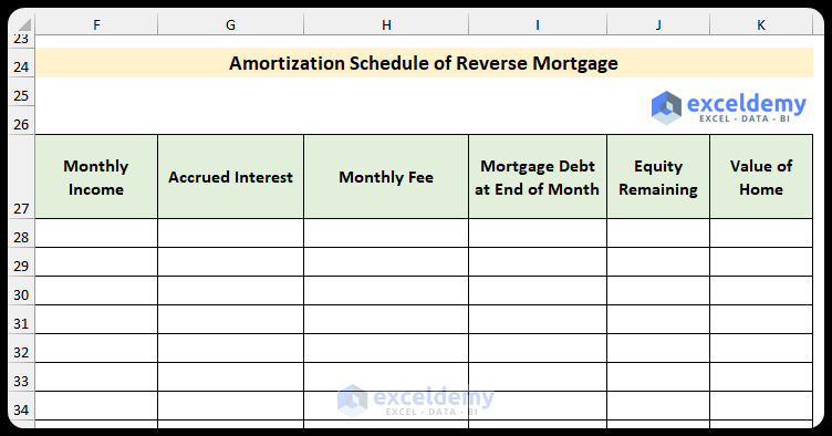
- Create these additional headers:
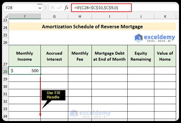
- Monthly Income
- Accrued Interest
- Monthly Fee
- Mortgage Debt at the End of the Month
- Equity Remaining
- Value of Home
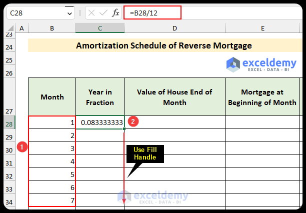
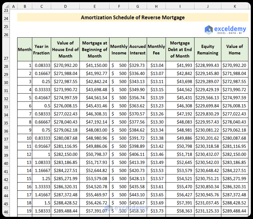
- Create a series in the month column, starting with 1. We created 777 rows as the example.
- Use this formula to convert the month values into the year values in the next column.
=B28/12
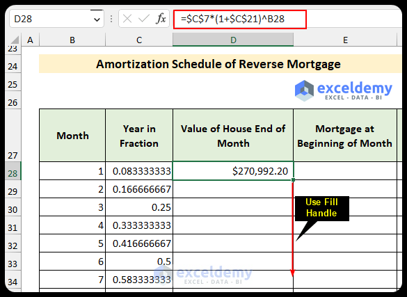
- Use this formula to find the value of the house at the end of the month, then use the Fill Handle to autofill the formulas.
=$C$7*(1+$C$21)^B28
- Use this formula to input the mortgage value at the beginning of the month in cell E28.
=C22
- Insert this formula in cell E29 to find the mortgage value at the end of the second month, then use the Fill Handle to apply the formula to the rest of the cells.
=I28
- Use this formula to find the monthly income.
=IF(C28<$C$10,$C$9,0)
- Insert this formula to calculate the accrued interest.
=(E28+F28)*$C$19
- Use the following formula to find the monthly fee.
=$C$14*(1+$C$20)^B28
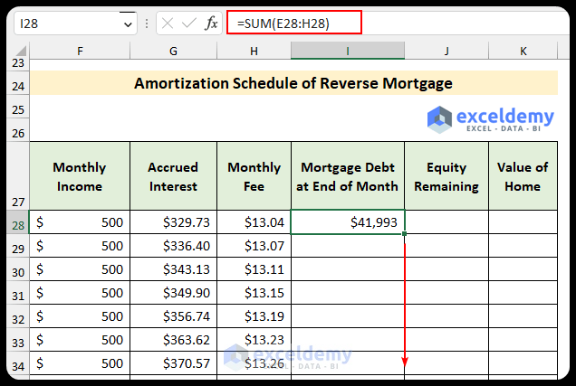
- This formula will return the mortgage debt at the end of the month.
=SUM(E28:H28)
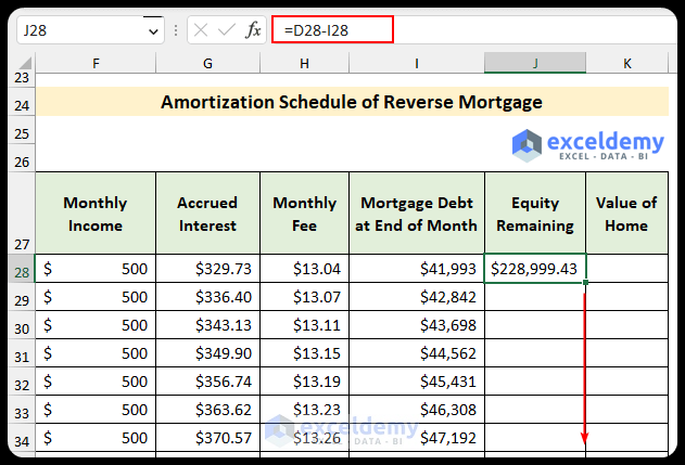
- Use this formula to find the remaining equity.
=D28-I28
- Insert this formula to find the value of the home.
=I28+J28
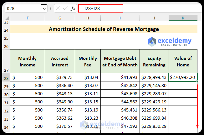
- The amortization schedule of the reverse mortgage will look like this.
- Insert this formula to calculate the years when the equity of the home falls to zero. The last value is in row 804, so we have used this in the formula.
=INT(COUNTIF(J28:J804,">0")/12)
Read More: Calculator for Effective Interest Method of Amortization
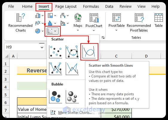
Step 4 – Plot Key Values
- From the Insert tab, select Scatter with Smooth Lines.
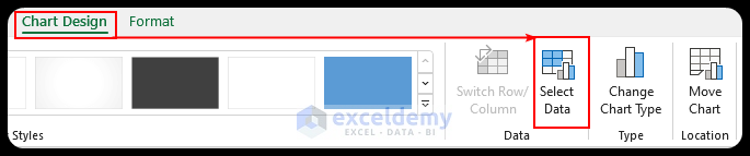
- Select the blank chart and, from the Chart Design tab, press on Select Data.
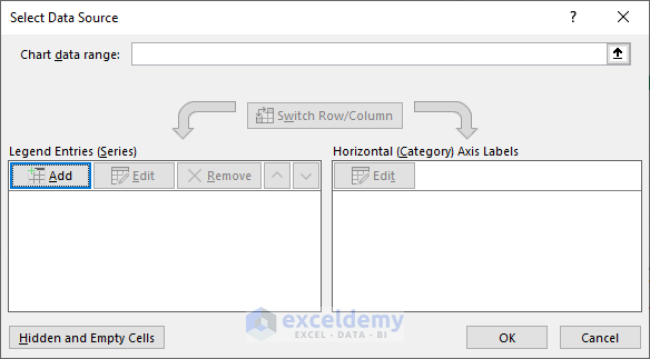
- Select Add from the Select Data Source dialog box.
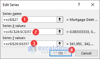
- Input the following values:
- Series name: cell I27.
- Series X values: Year in Fraction.
- Series Y values: value from the Mortgage Debt at End of Month column. We have included the values up to the cell where the equity remains positive which is row 357. Moreover, “ss!” means the data is in the “ss!” sheet.
- Press OK.
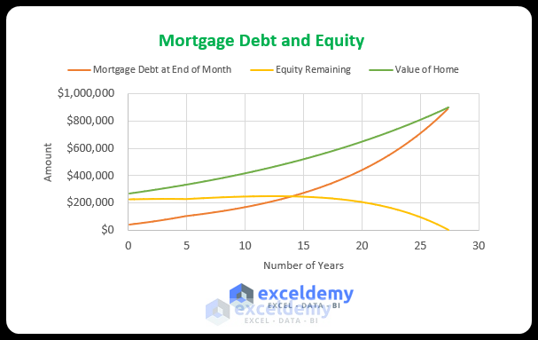
- A curved line will appear in the chart.

- Repeat the above process for the “Equity Remaining” and “Value of Home” columns.
- Wwe can see that after 27 years, the equity becomes zero.
Read More: Mortgage Calculator with Extra Payments and Lump Sum in Excel
Download the Template
Related Articles
- How to Create Offset Mortgage Calculator in Excel
- Early Mortgage Payoff Calculator in Excel
- Mortgage Repayment Calculator with Offset Account and Extra Payments in Excel
- How to Make Chattel Mortgage Calculator in Excel
- Creation of a Mortgage Calculator with Taxes and Insurance in Excel
- Interest Only Mortgage Calculator with Excel Formula
- Biweekly Mortgage Calculator with Extra Payments in Excel
<< Go Back to Mortgage Calculator | Finance Template | Excel Templates
Get FREE Advanced Excel Exercises with Solutions!

Would it be possible to have a column that would include extra repayments, regular and lump sum, as well as redraw? A bit like a LOC. I guess that would be far more complicated to consider when in the month that would occur?
Thank you.
Hello Brin,
Yes, this is definitely possible, but it would require a few enhancements to the existing amortization table.
You can extend the current setup by adding additional columns such as Regular Extra Repayment, Lump Sum Payment, and Redraw. Then, the balance calculation in each period would need to be adjusted to account for these values. The key part is maintaining the correct sequence within each month—typically applying redraw (if any), then calculating interest, and finally subtracting scheduled and extra repayments.
So while the current template focuses on the standard reverse mortgage calculation for simplicity, it can absolutely be customized to handle these more advanced scenarios with a bit of restructuring.
Regards,
ExcelDemy