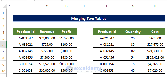
How to Merge Two Tables in Excel (5 Methods)

We will use the following dataset to create a relationship between the two tables in Excel with duplicate values. Both of the data sets have a common column. The common column is Product ID.

How to Merge Two Tables in Excel

Method 1 – Using the VLOOKUP Function to Merge Two Tables in Excel

Steps

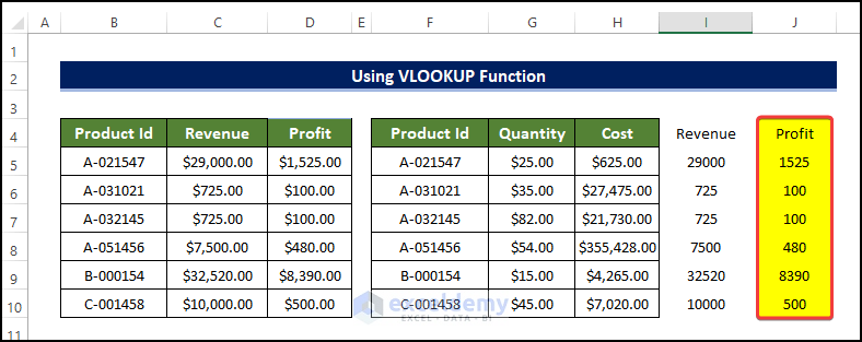
The common column is the Product ID column.

Using VLOOKUP Function to Merge Two Tables in Excel

Select the cell I4 and enter the following formula:

=VLOOKUP(F4,$B$4:$D$10,2,FALSE)

vlookup formula input

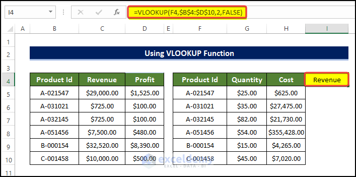
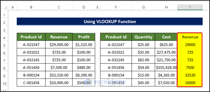
Drag the Fill Handle to cell I10.
This will fill the range of cell I4:I10 with the second column of the first table.

one column merge between two tables

Select cell J4 and enter the following formula:

=VLOOKUP(F4,$B$4:$D$10,3,FALSE)

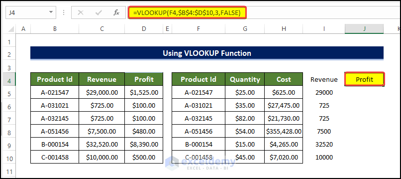
vlookup formula input for second column .

Drag the Fill Handle to cell J10.

Select a range of cells D4:D10, then click on the format painter icon from the Clipboard group in the Home tab.
A small paint brush appears in the place of the cursor.
Select the range of cells I4:J10.

formatted the output

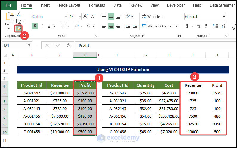
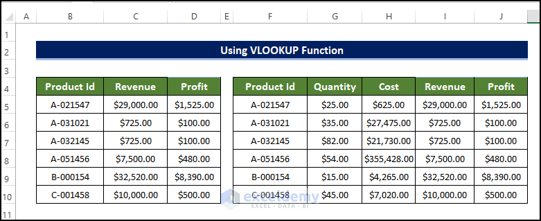
The two tables are now merged and formatted.

two separate table merge using functions.

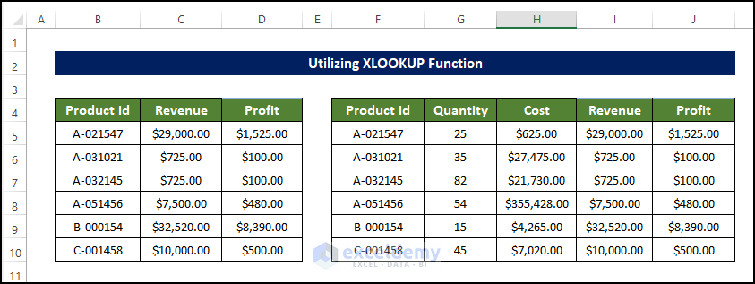
Method 2 – Applying the XLOOKUP Function to Merge Two Tables

Steps

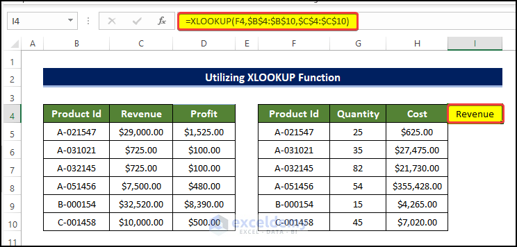
For the given tables, the common column is the Product ID column.

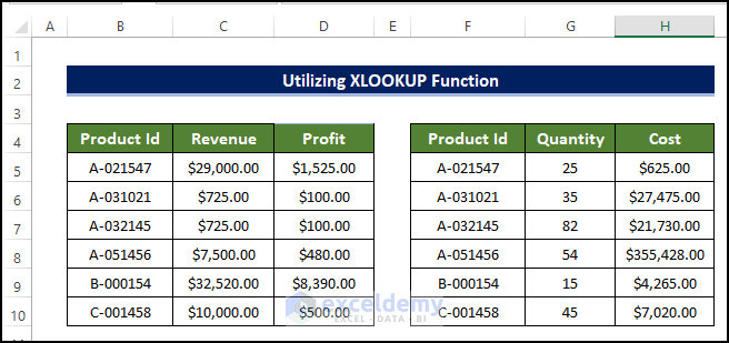
Utilizing XLOOKUP Function to Merge Two Tables in Excel

Select the cell I4 and enter the following formula:

=XLOOKUP(F4,$B$4:$B$10,$C$4:$C$10)

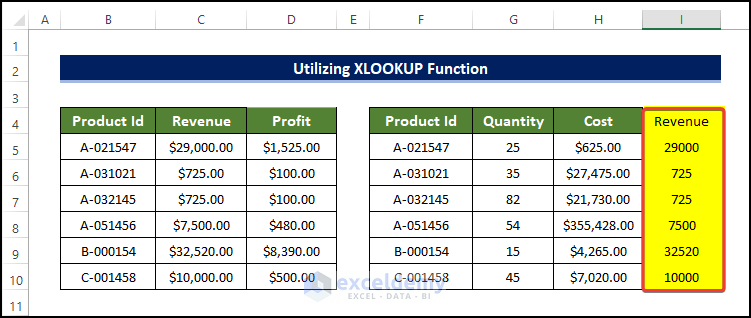
Drag the Fill Handle to cell I10.

first column merged

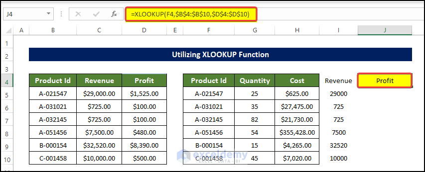
Select the cell J4 and enter the following formula:

=XLOOKUP(F4,$B$4:$B$10,$D$4:$D$10)

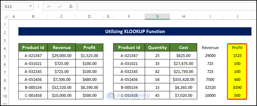
XLOOKUP formula input to merge two tables

Drag the Fill Handle to cell J10.

second column is merged

Select a range of cells D4:D10 and click on the format painter icon from the Clipboard group in the Home tab.
A small paintbrush appears in the place of the cursor.
Select the range of cells I4:J10.

output formatting

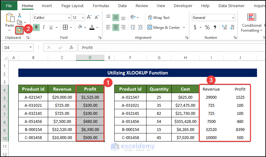
You can see the two tables are now merged and formatted.

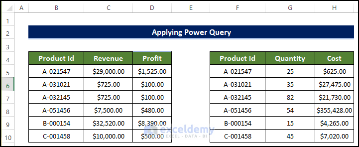
merge two enage of cells by matching values

Method 3 – Merging Two Tables with Excel Power Query

Steps

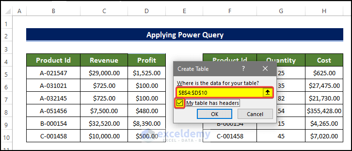
The common column is the Product ID column.

Applying Power Query to merge two tables in excel

Go to Data and select Get Data.
Pick From Other Sources and choose From Table/Range.

Input table to power query

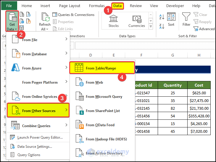
A small dialog box will appear.
Enter the range of the first table and tick the My table has headers box.
Click OK.

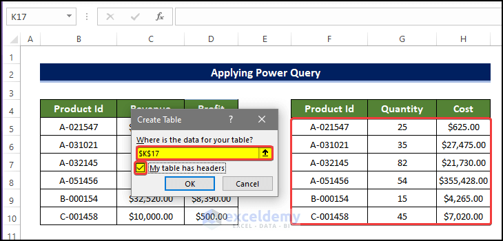
Repeat the process for the second table.
In the Power Query, create a table dialog box, specify the range of the table, and tick the check box My table has headers.
Click OK after this.

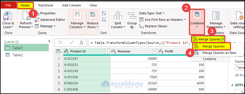
Open the power query editor (clicking OK in the previous step will automatically launch the editor).
Go to the Home tab.
Go to the Combine group.
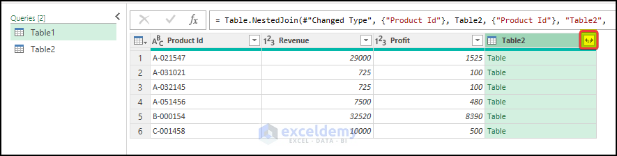
Click on the Merge Queries.
From the drop-down menu, click on the Merge Queries.

merge queries using combine

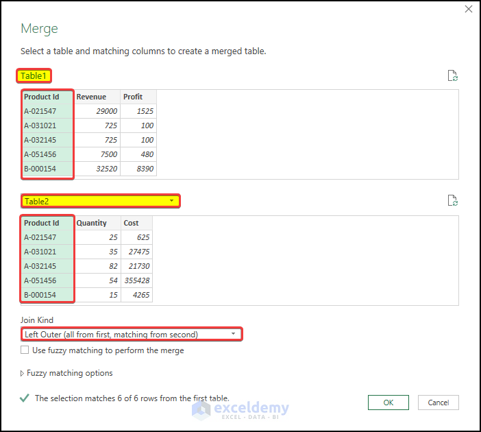
In the new window named Merge, choose Table 1 as the first table
Choose Table 2 as the second table.
Choose Left Outer (all from the first, matching from the second).
Click OK.

selection of the merged table

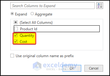
Click on the top-right corner of the Table2 column header.

expanding merged table

Check the Quantity and Cost boxes, as we already have the Product Id in the first table.
Uncheck the Use Original Column name as a prefix box.
Click OK after this.

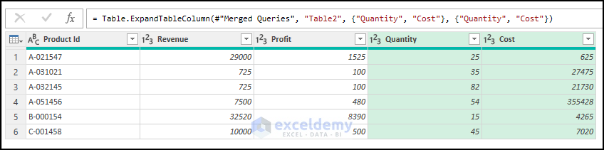
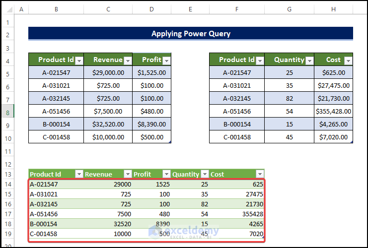
Two columns are now added to the first table.

combine command to merge tables

Click on Close and Load from the Home tab.
From the drop-down menu, click on Close and Load To.

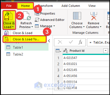
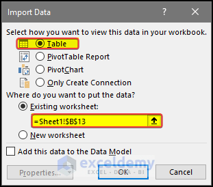
load the two merge table to the worksheet.

Select Table in the Select how you want to view this data in your workbook
Choose Existing worksheet and select cell B13.
Click OK.

The table will be loaded into cells B13:F19.

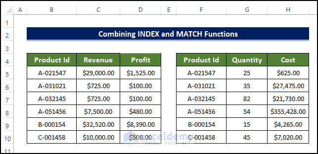
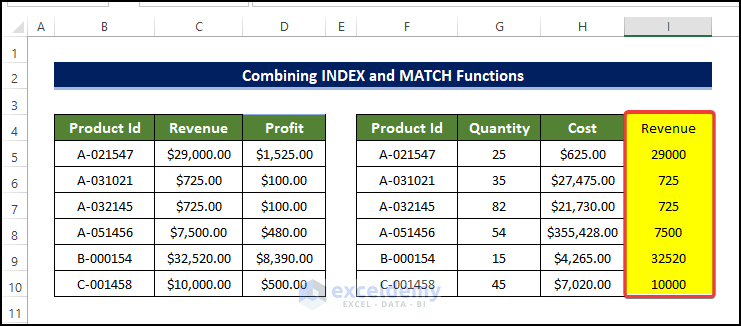
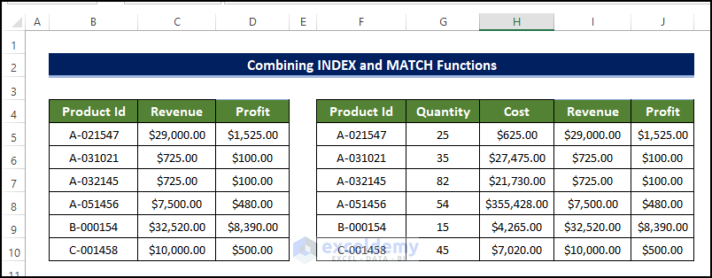
merging queries to merge two tables

Method 4 – Combining INDEX and MATCH Functions

Steps

The common column is the Product ID column.

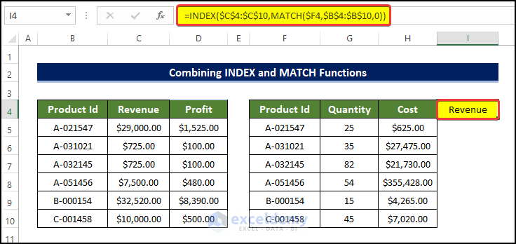
Combining INDEX and MATCH Functions to Merge Two Tables in Excel

Select the cell I4 and enter the following formula:

=INDEX($C$4:$C$10,MATCH($F4,$B$4:$B$10,0))

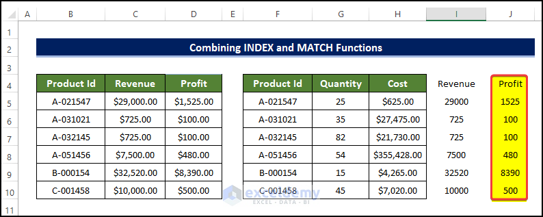
Drag the Fill Handle to cell I10.

first column of the first table are merged to second column

Select cell J4 and enter the following formula:

=INDEX($D$4:$D$10,MATCH($F4,$B$4:$B$10,0))

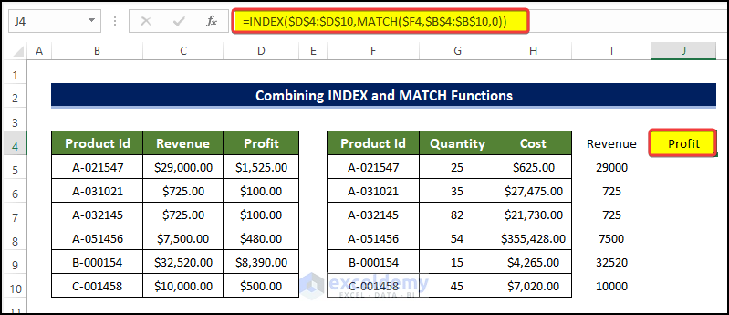
Drag the Fill Handle to cell J10.

merging the second column of the first table

Select a range of cells D4:D10 and click on the format painter icon from the Clipboard group in the Home tab.
A small paintbrush appears in the place of the cursor.
Select the range of cells I4:J10.

formatting the output

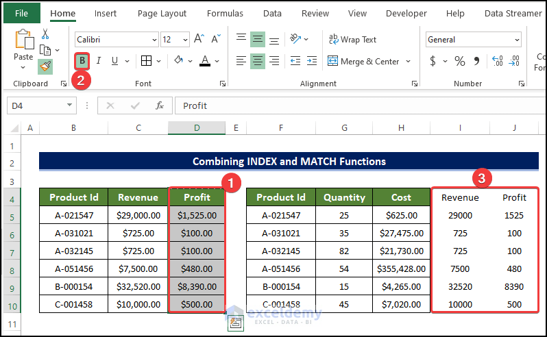
The two tables are now merged and formatted.

Formula Breakdown

MATCH($F4,$B$4:$B$10,0)

This function will look for the exact value specified in the first argument in the array/ range of cells mentioned in the second argument. In this case, it will look for the value in the cell F4 in the lookup array in the B4:B10, and return the serial of that value in that range.

INDEX($C$4:$C$10,MATCH($F4,$B$4:$B$10,0))

After we get the serial of the matched value in the lookup array, the formula will look for the value of the same serial in the other column (first argument) in the table.

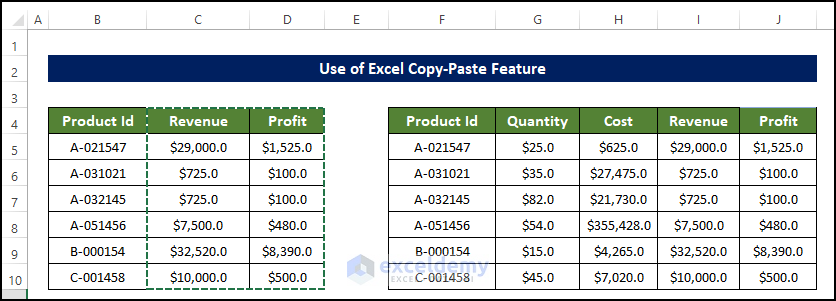
Method 5 – Using Excel Copy-Paste to Merge Two Tables

Steps

Sort the tables based on the matching column. The respective column of both tables need to contain the same values.

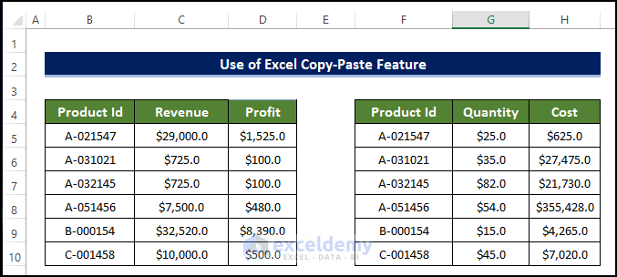
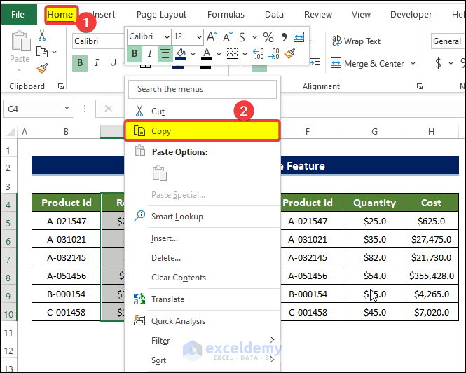
Use of Excel Copy-Paste Feature to Merge Two Tables in Excel

Select the second and the third column of the first column and right-click.
From the context menu, click on Copy.

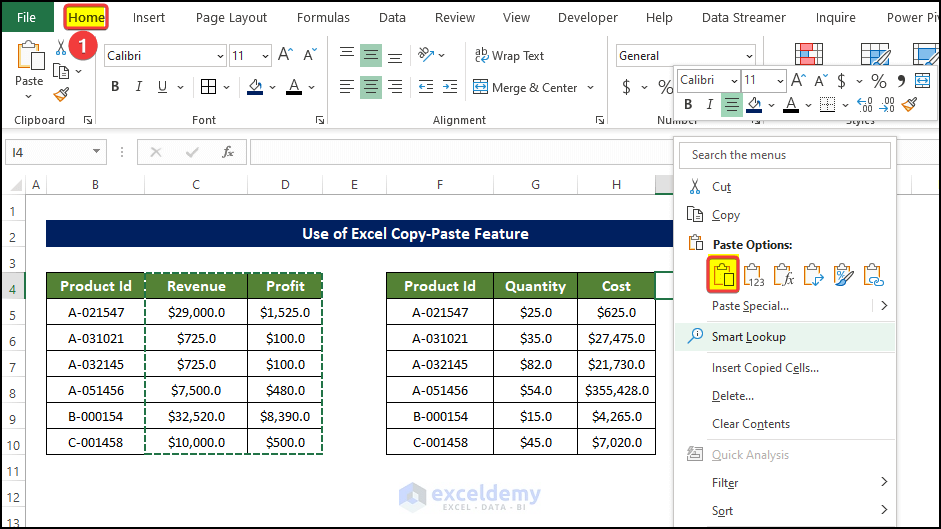
Select cell I4 and right-click on it.
Click on Paste.

pasting copied cells

Pasting the first table columns into the second table column will merge the two tables.

copy and paste to merge two tables

Things to Remember

You need to maintain the same serial numbers for the column entries in the common columns in both of the tables.
In the Power Query method, use the left-most table as the first.

Download the Practice Workbook

Merge Two Tables.xlsx

<< Go Back to Merge Tables in Excel | Merge in Excel | Learn Excel

Get FREE Advanced Excel Exercises with Solutions!