Excel is the most widely used tool for dealing with massive datasets. We can perform myriads of tasks of multiple dimensions in Excel. Excel provides us with different ways to calculate using various functions. For example, we can use explicit cell references or structured references in Excel. This article will show you how to use IF function and structured reference in Excel.
Introduction to Structured Reference
The syntax for referencing Excel Tables is known as a structured reference. Excel gives the table and each column heading it contains a name when you create an Excel table. When adding formulas to an Excel table, you can choose the references from the table. When you use structured reference, the column names will pop up despite a particular cell. Every time you add or remove data from the table, the names in structured references change because of their dynamic nature.
How to Use IF Function and Structured Reference in Excel: 2 Easy Steps
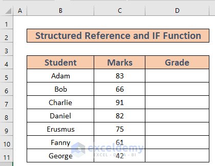
This is the dataset for today’s article. We have some students and their marks in a particular subject. I am going to assign the grades using the IF function. More to that, I will use the structured reference while applying the formula.
Step 1: Create Table with Proper Data
First of all, I will create a table with the entire dataset. This is a requisite to use structured references. For this,
- Select the range B4:D11.
- Then, go to the Insert.
- After that, select Table.

- Create Table box will appear. Check My table has headers box as the table has headers.
- Then, click OK.
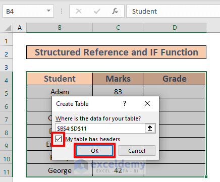
- Excel will create a table.

Step 2: Apply Formula Using IF Function
Now, I will use the IF function to assign grades to the students. Let’s see how to do it.
- Go to D5 and write down the following formula:
=IF([@Marks]>=90,"A",IF([@Marks]>=80,"B",IF([@Marks]>=70,"C",IF([@Marks]>=60,"D","F"))))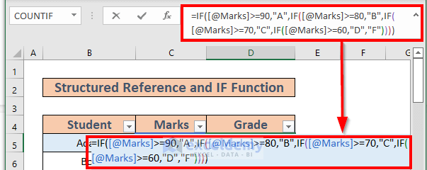
Note: [@Marks] appears because the D4:D11 range is a table. That’s why Excel is using the structured reference i.e., selecting the entire column when you select a single cell (C5) under the Marks column.
Explanation:
The value in D5 is 81.
- Excel tests the logical tests one by one. First, it tests [@Marks]>=90.
- [@Marks]>=90 is FALSE. That’s why it checks the next logical test. That is [@Marks]>=80.
- [@Marks]>=80 is TRUE. So, Excel will return the output “B”.
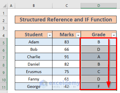
- Now, press ENTER. Excel will return the output.

- Now, use the Fill Handle to AutoFill up to D11.
Read More: How to Reference a Dynamic Component of a Structured Reference in Excel
Things to Remember
- When using Nested IF, please remember that Excel will first check the first logical test. If the test is FALSE, Excel will check the 2nd one, and so on. But if the 1st test is TRUE, Excel will stop checking other conditions and get you the output for the 1st logical test.
- You can use CTRL+T as a keyboard shortcut to create a table after selecting the range.
Download Practice Workbook
Download this workbook and practice while going through this article.
Conclusion
In this article, I have shown you how to use IF function and structured reference in Excel in easy steps. I hope it helps everyone. If you have any suggestions, ideas, or feedback, please feel free to comment below.
Related Articles
- How to Lock a Structured Reference in Excel
- What is an Unqualified Structured Reference in Excel?
- How to Use HLOOKUP with Structured Reference in Excel
- Applications of Absolute Structured References in Excel Table Formulas
<< Go Back to Structured Reference | Table Formula | Excel Table | Learn Excel
Get FREE Advanced Excel Exercises with Solutions!
