How to Use HLOOKUP with Structured Reference in Excel

What Is a Structured Reference?

A structured reference is a term that refers to using a table name in an Excel formula in lieu of a usual cell reference. We will consider it an absolute structured reference if the table name that we are using as a reference does not change when we copy the formula to another cell. The default syntax for absolute structured reference is:

Table[[Column_1]:[Column_2]]

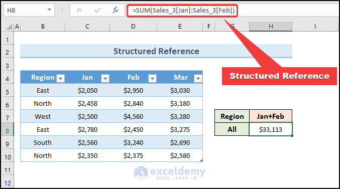
For instance, we have selected the output cell H8 and typed the following formula to get the total value of January and February using the SUM function.

=SUM(Sales_3[Jan]:Sales_3[Feb])

The following image indicates the overview of structured references.

How to Use HLOOKUP with a Structured Reference in Excel: 5 Suitable Examples

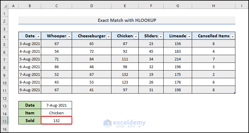
Example 1 – Exact Match with HLOOKUP

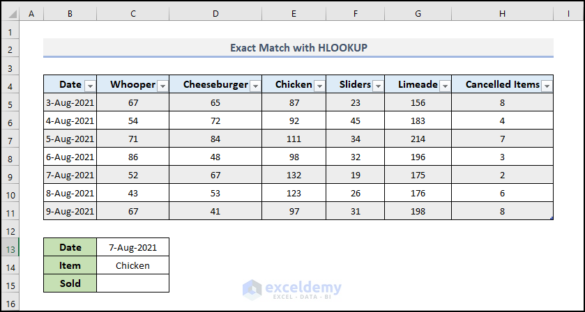
Using the chart or table below, we can see how many people have ordered certain foods on a given day over time. Column H lists the total number of items or orders that were canceled on each of those days. We can find out how many fried chickens were sold in that restaurant on August 7th, 2021.

Steps:

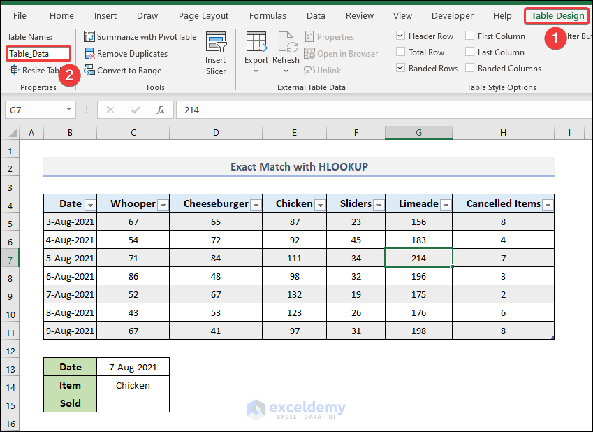
Select any cell randomly from the table range.
Go to the Table Design tab and type a name in the Table Name field. We named the table ‘Table_Data’. We will use this table name as a reference in the formula.

Select the output cell C15 and use the following formula.

=HLOOKUP(C14,Table_Data[#All],6,FALSE)

C14 represents the lookup value, and ‘Table_Data [#All]’ illustrates the Table Array. The third argument is the row number, which corresponds to August 7, 2021, in the table. In the 4th argument of the HLOOKUP function, we have defined the range_lookup as FALSE, which means the function will search for the exact match of the lookup item, ‘Chicken’ in the table.

Press Enter.

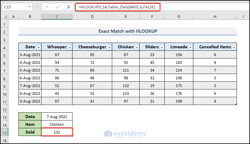
The function will return 132. So, a total of 132 pieces of fried chicken were sold on that particular date.

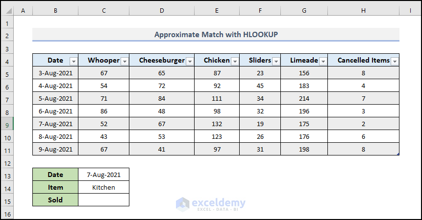
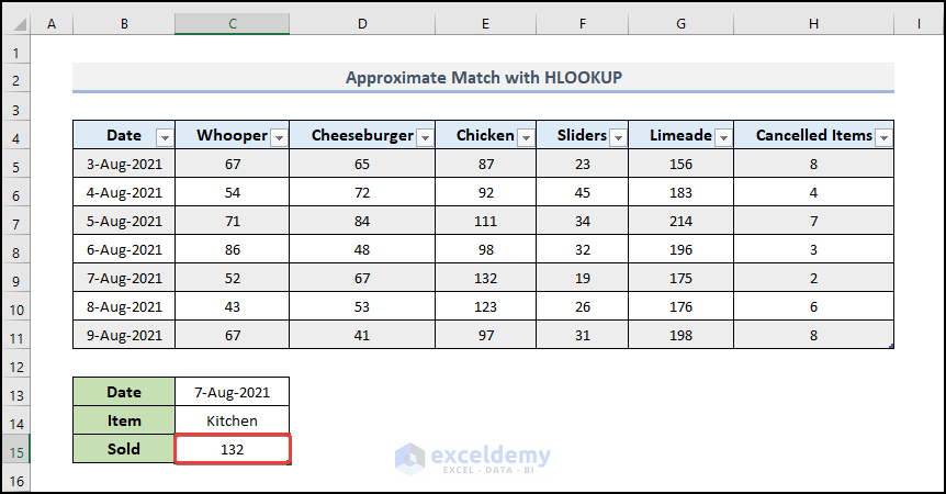
Example 2 – Approximate Match with HLOOKUP

By setting the fourth argument to TRUE, the HLOOKUP function can be used with Approximate Match. If our search criteria partially match the desired exact name, the function will return the output cell if the exact data is located.

Steps:

Select any cell randomly from the table range.
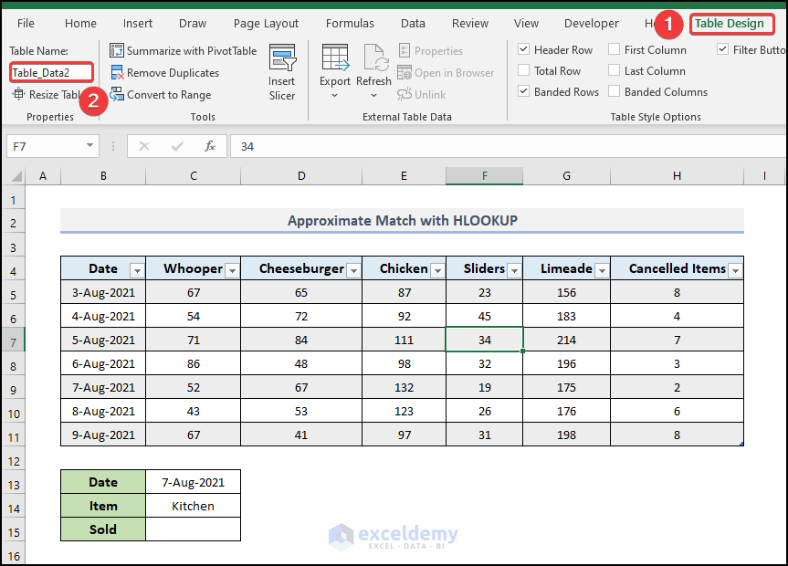
Go to the Table Design tab and type a name in the Table Name field. We named the table ‘Table_Data2’.

Select the output cell C15 and use the following formula.

=HLOOKUP(C14,Table_Data2[#All],6,TRUE)

C14 represents the lookup value, and ‘Table_Data2 [#All]’ illustrates the Table Array. By using TRUE in the 4th argument, we’ve just got a match even after we’ve typed the name of a wrong item that is absent from the table. In cell C14, you can now enter additional food names or partially matched names from the table and observe the function’s output.

Press Enter.

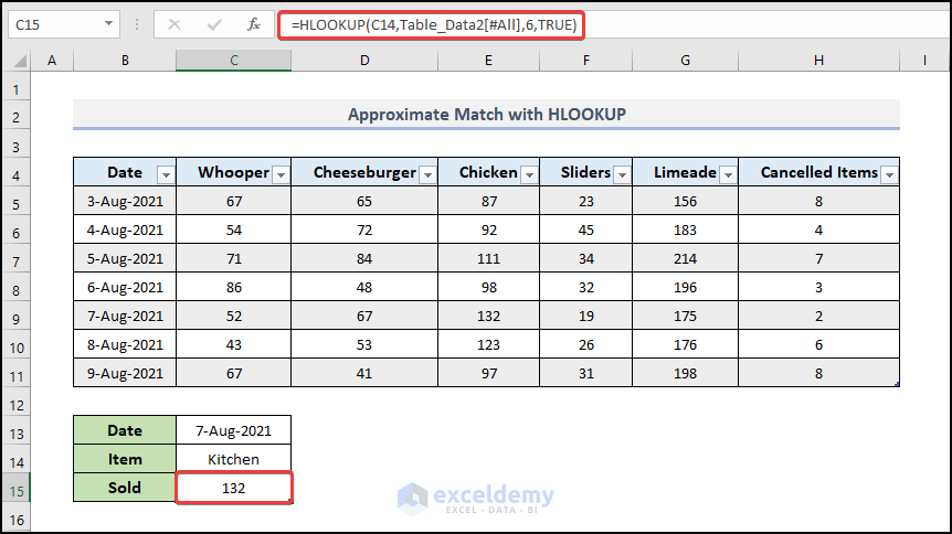
We got the value of 132.

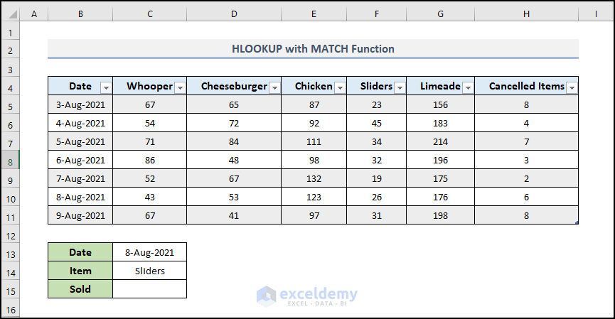
Example 3 – HLOOKUP with MATCH Function

If you don’t want to repeatedly define the row number within the HLOOKUP function, but need to change the date or value in cell C13 and obtain an immediate result, you must use the MATCH function to define the row number of the data present in the corresponding cell. Cells C13 and C14 display, respectively, the date and the food item.

Steps:

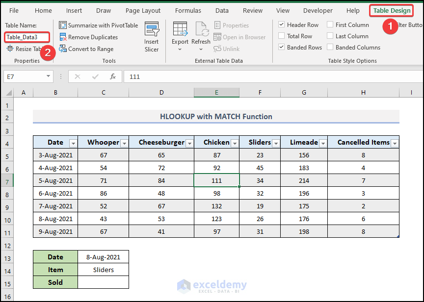
Go to the Table Design tab and type a name in the Table Name field. We named the table ‘Table_Data3’.

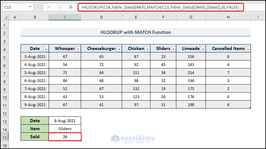
Select the output cell C15 and use the following formula.

=HLOOKUP(C14,Table_Data3[#All],MATCH(C13,Table_Data3[[#All],[Date]],0),FALSE)

The output will update whenever you change the date or name of the food item in cells C13 and C14.

Press Enter.

Here’s the result.

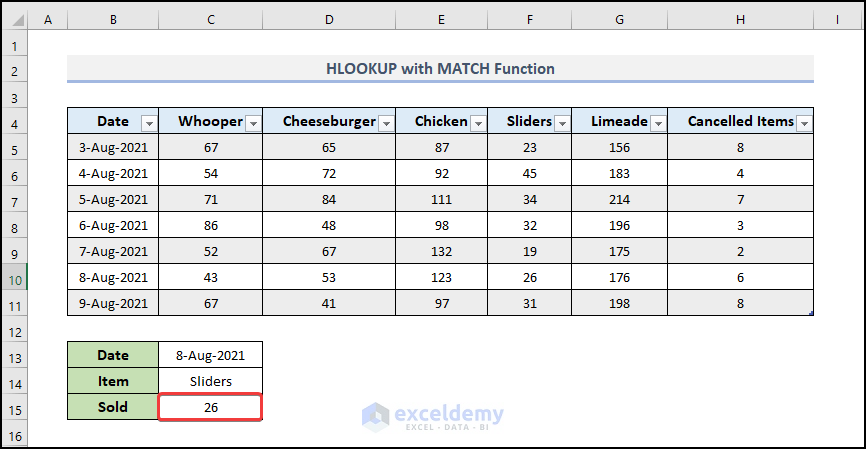
How Does the Formula Work?

MATCH(C13,Table_Data3[[#All],[Date]],0)

C14 represents the lookup value, and ‘Table_Data3 [#All]’ illustrates the Table Array. Here, the MATCH function defines the row number of the data present in the corresponding cell. This function will produce the position of C13 in the array and return 7.

HLOOKUP(C14,Table_Data3[#All],MATCH(C13,Table_Data3[[#All],[Date]],0),FALSE)

Cells C13 and C14 display, respectively, the date and the food item. In the 4th argument of the HLOOKUP function, we have defined the range_lookup as FALSE, which means the function will search for the exact match of the lookup item- ‘Sliders’ in the table and return 26.

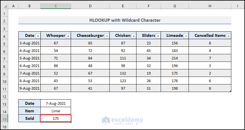
Example 4 – HLOOKUP with a Wildcard Character

On 7 August 2021, we want to find out how many orders were placed for a food item that contained the text ‘Lime’.

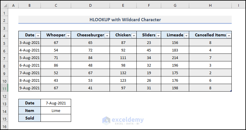
Steps:

Go to the Table Design tab and type a name in the Table Name field. We named the table ‘Table_Data4’.

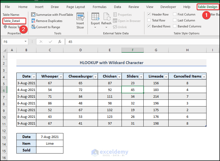
Select the output cell C15 and use the following formula.

=HLOOKUP("*"&C14&"*",Table_Data4[#All],6,FALSE)

C14 represents the lookup value, and ‘Table_Data [#All]’ illustrates the Table Array. In the 4th argument of the HLOOKUP function, we have defined the range_lookup as FALSE, which means the function will search for the partial match of the lookup item- ‘Lime’ in the table.

Press Enter.

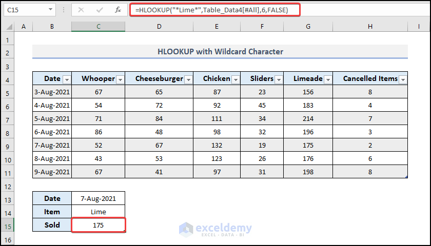
Here’s the result.

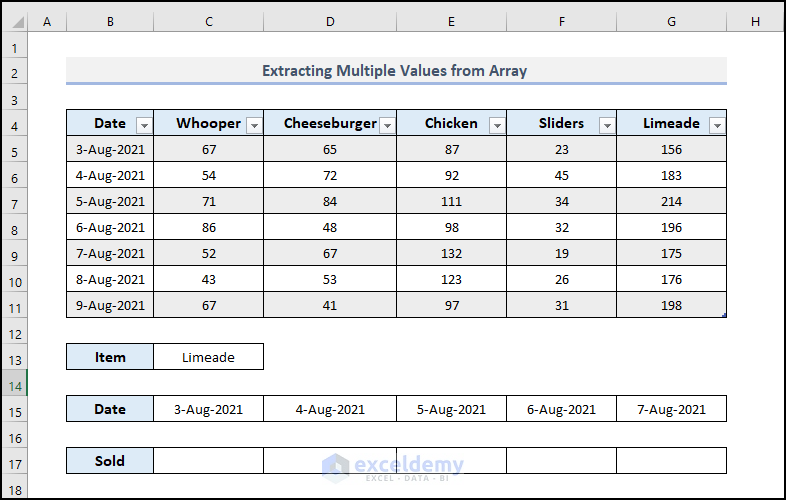
Example 5 – Extracting Multiple Values from an Array

We will determine the quantity of limeade sold over a 5-day period starting on August 3, 2021.

Steps:

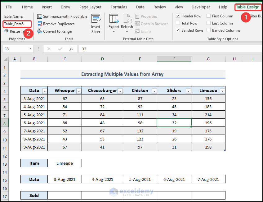
Go to the Table Design tab and type a name in the Table Name field. We named the table ‘Table_Data5’.

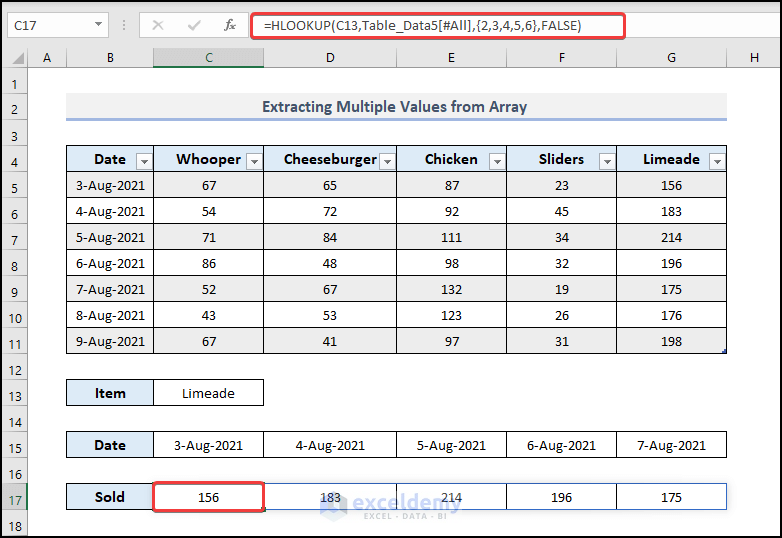
Select the output cell C15 and use the following formula.

=HLOOKUP(C13,Table_Data5[#All],{2,3,4,5,6},FALSE)

C13 represents the lookup value, and ‘Table_Data5 [#All]’ illustrates the Table Array. In the 4th argument of the HLOOKUP function, we have defined the range_lookup as FALSE, which means the function will search for the partial match of the lookup item- ‘Limeade’ in the table.