When you create a chart in Excel, the data series is named automatically. You might occasionally need to change the name of the data series for personal or professional reasons. In this blog post, you will learn how to rename series in Excel.
How to Rename Series in Excel: 3 Suitable Examples
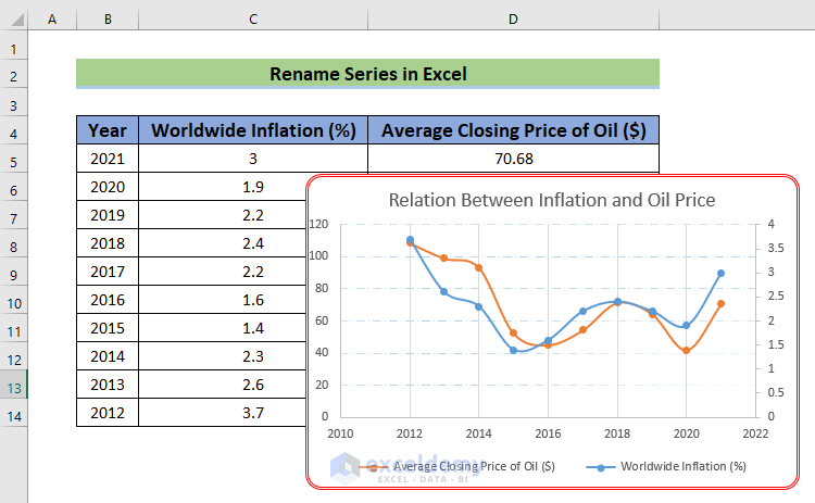
Excel provides a few options for renaming data series. We have created a dataset with the column titles Year, Global Inflation (%), and Average Closing Price of Oil ($) to demonstrate this. The sample data set is shown below:
1. Rename a Data Series in Excel
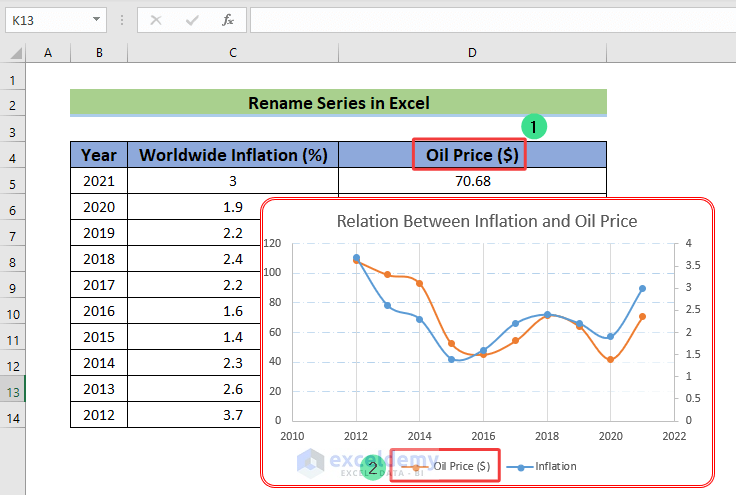
By editing the dataset, especially the column headings that serve as the chart’s legends, we may change the legends. The following dataset and chart, where the columns are Year, Worldwide Inflation (%), and Average Closing Price of Oil ($), is what we’re going to use. These legends require new names.
📌 Steps:
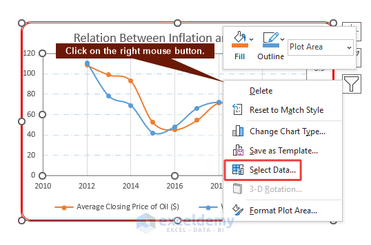
- To choose data, use the right-click menu to select the chart whose data series you want to rename. See illustration:
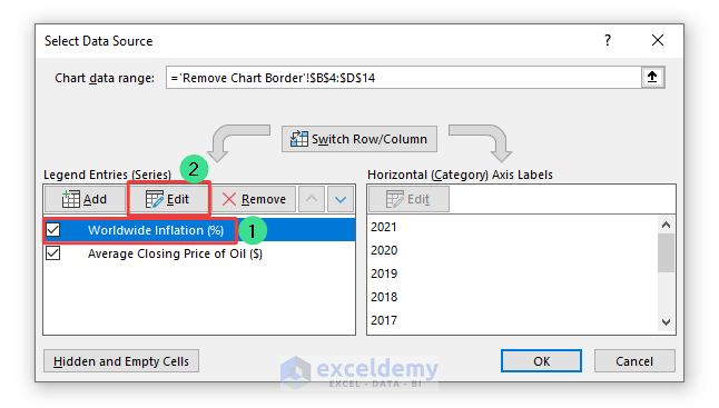
- A Select Data Source dialog box appears at this point. Please choose the data series that you want to rename by clicking upon that, and then select the Edit option. See illustration:
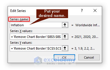
- Feel free to delete the previous series name from the Edit Series dialog box before typing the new series name inside the Series name field and clicking the OK option. See illustration:
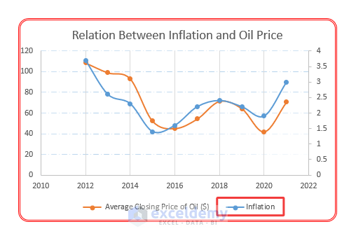
- Note that the legend name has been changed to Inflation only like the image below.
2. Rename Series Legends by Double Clicking on Them
We may rename the legends by editing the dataset, especially the column headings that serve as the chart’s legends.
📌 Steps:
- To begin, double-click the D4 cell and alter Oil Price ($) as the column header.
- Next, key in ENTER.
- At some point, we’ll notice that the chart’s initial legend has been modified to read Oil Price ($).
3. Rename Axis Title of a Series
Sometimes, you may not have legends or axis titles when you first create the graph from the data. We are going to show the necessary steps in the following steps:
📌 Steps:
- Firstly, we will select the data and then click on the Plus sign beside the chart. After that select the preferred option according to your project.
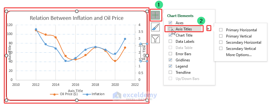
- Notice in the image that, we have added the % and $ signs by editing the Axis Title like the image below.

Read More: How to Format Data Series in Excel
Download Practice Workbook
You can download the practice workbook from the following download button.
Conclusion
Follow these steps and stages to understand the topic of how to rename a series in Excel. You are welcome to download the workbook and use it for your own practice.
Related Articles
<< Go Back To Data Series in Excel | Excel Charts | Learn Excel
Get FREE Advanced Excel Exercises with Solutions!
