How to Add Data Series in Excel Chart (2 Easy Methods)

In this article, I am going to show how we can add data series in Excel chart. The data series refers to a row or column containing numbers that are used to plot charts in Excel. While inserting a chart in Excel, sometimes Excel misses out on an adjacent column or row and plots the chart without it. In addition to that, after inserting a chart, a user may need to add another row or column to plot in the same Excel chart.

In this article, we will learn how to add adjacent column or row data series to an existing Excel chart. We will also see, how to add any column or row data series to an Excel chart.

Download Practice Workbook

Download this practice workbook to exercise while you are reading this article.

How to Add Data Series to a Chart in Excel: 2 Easy Methods

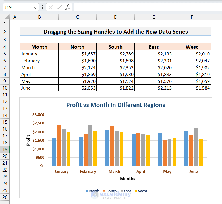
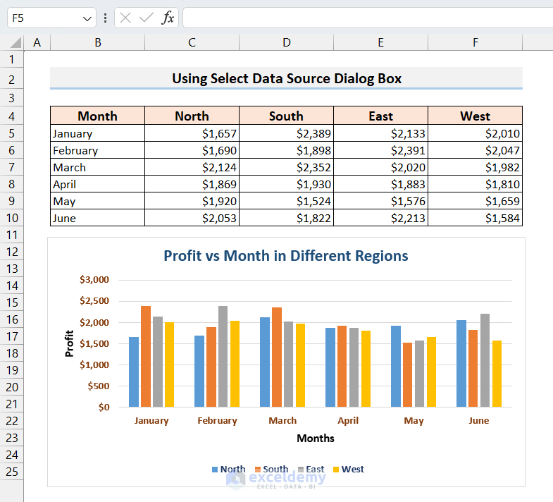
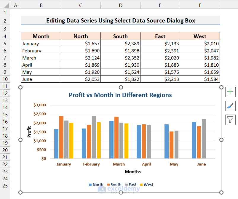
In this section, we will demonstrate 2 effective methods for adding data series to a chart in Excel. For this illustration purpose, I have taken a data set containing the profit of different regions of a company by month. I also inserted a column chart using the data set.

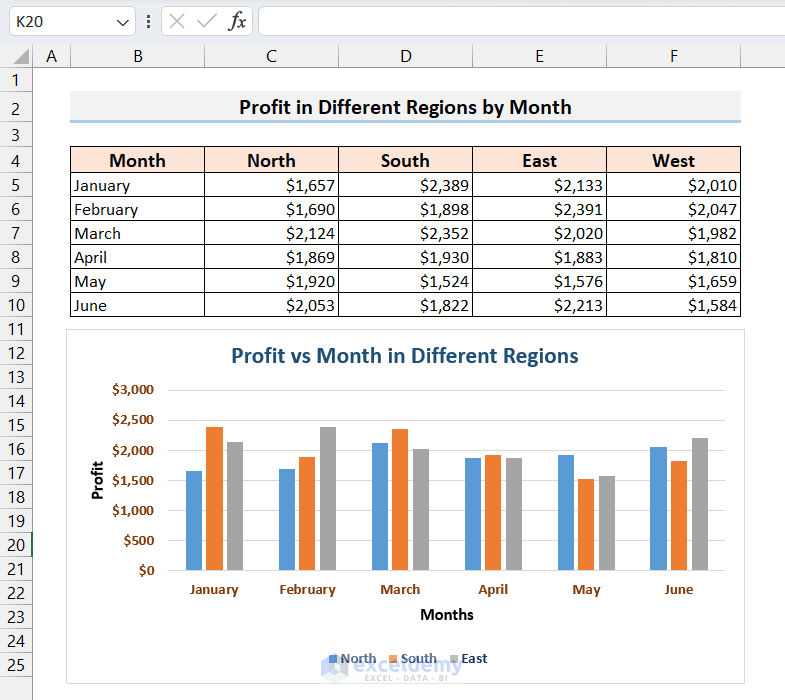
From the chart, we can see that the West column data series was somehow not included in the chart. Hence, we will try to add the West data series.

1. Dragging the Sizing Handle to Add New Data Series

If the new data series that we need to add to a chart is adjacent, then we can use the sizing handle to easily incorporate the new series. To do that, follow the steps below.

• First, click on anywhere on the chart. As a result, you will see that the existing data series are being highlighted.

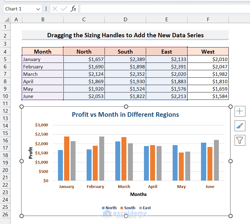
• Now, bring the mouse cursor to the bottom right corner of the highlighted data series. As a result, you will see the sizing handle. Now, drag the sizing handle to the right to include the West

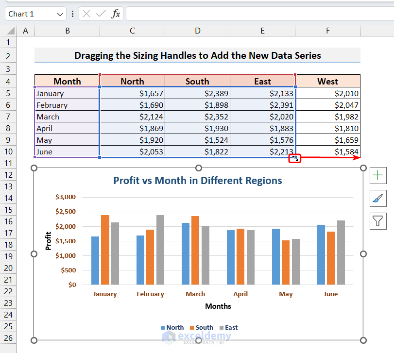
• Consequently, the west data series will be added to the chart.

In this way, we can easily add multiple new data series that are adjacent to the existing data series.

2. Using Select Data Source Dialog Box

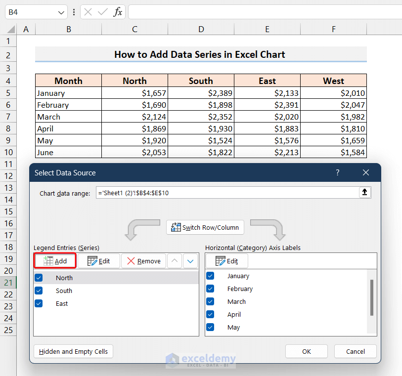
In the previous method, we saw how to add any adjacent data series to an Excel chart. But in many situations, the new data series may not be adjacent to the previously used data series. Hence, in that situation, instead of using the Sizing Handle, we need to use the Select Data Source dialogue box. To learn more, follow the steps below.

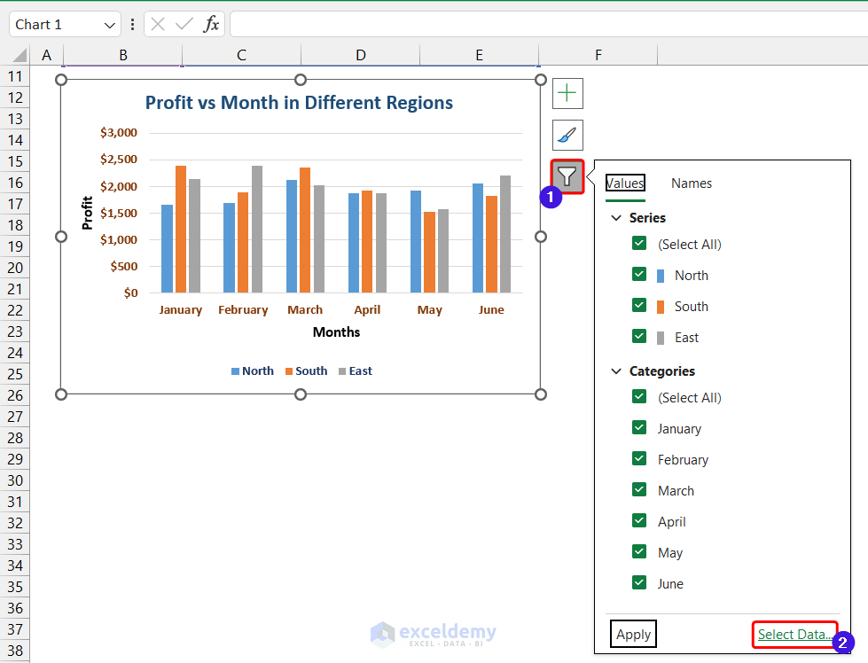
• First, click anywhere on the chart. As a result, a context menu on the right side of the chart will appear. From that menu, click on Filter.  Now, from the menu that appears on the right side, click on the Select Data option at the bottom.

• From the Select Data Source dialogue box, click on the Add option.

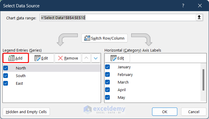
• As a result, a new window named Edit Series will open up. From the window, select the range of Series name and Series value. Here, we can select any range from any worksheet in the workbook. After that, click OK.

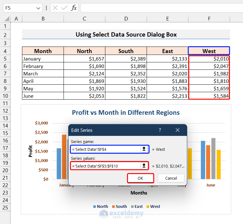
• As a result, the new data series will be added to the chart.

In this way, we can easily add as many data series as we want.

How to Edit Data Series of a Chart in Excel

After adding a data series, we may want to change or modify the value range or name of the series. To do that, we can also use the Select Data Source dialog box. To learn more, follow the steps below.

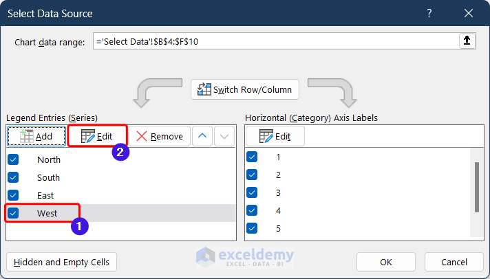
• By following the same procedure described in the 2nd method, open the Select Data Source dialog box. In this window, you will see the list containing all the data series. From there, select any data series that you want to edit and click on the Edit option.

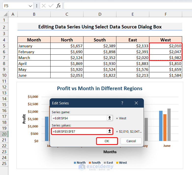
• Next, a new window named Edit Series will open up. In the window, you can again select the range for series name and series values. After editing them, click OK.

• After that, in the Select Data Source dialog box, again click OK.

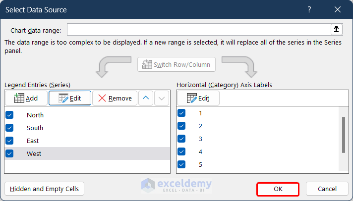
• As a result, the edited data series will be saved, and the edited chart will be displayed.

Alternative Way for Editing Data Series

There is another smart way to edit data series. In this method, first, we need to click on any column of the series that we want to edit in the chart. For example, I am selecting the East Column. As a result, the formula of that data series will be displayed in the formula box.

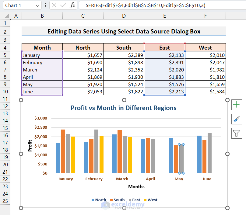
• Here is the displayed formula :

• In the formula, there are four arguments. The 1st argument takes the range for the series name, the 2nd argument takes X-axis values, the 3rd argument takes the Y-axis value and the 4th argument takes the position of the data series in the chart.
• By editing the range in the formula, we can directly change the data series.

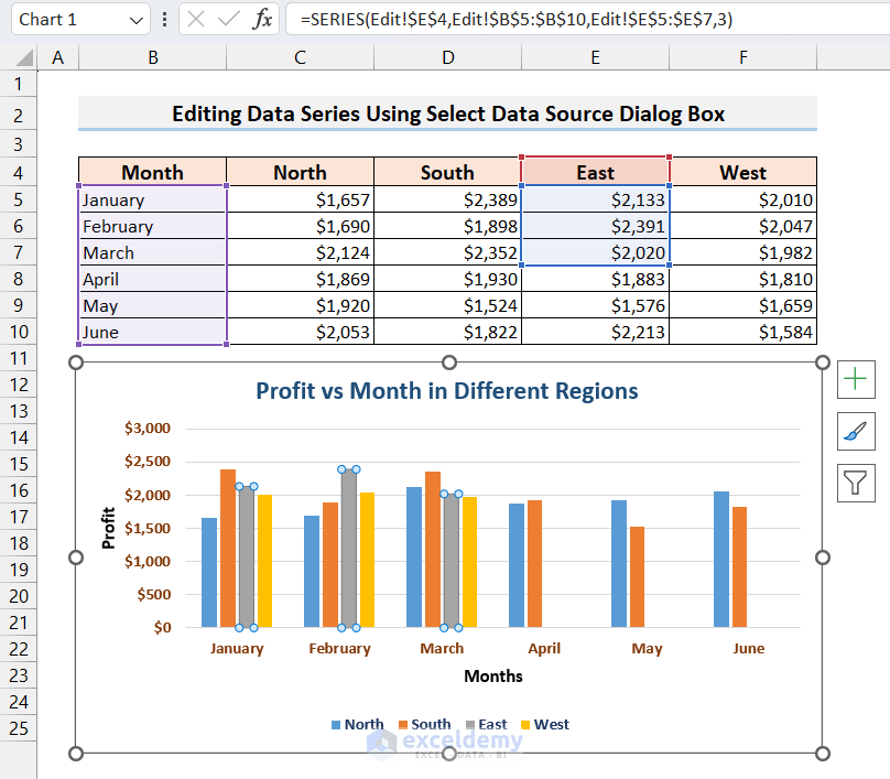
Things to Remember

• The first method can only be applicable when the new data series is adjacent to the prior used series.
• In the second method, we can also open the Select Data Source dialogue box from the Chart Design tab on the ribbon.

Frequently Asked Questions

1. Where is data series in Excel?

In Excel, a “data series” refers to a set of related data points that are plotted in a chart. Each data series is represented on the chart by a unique set of data points, and they all share a common property.

2. How do I create a data series in Excel?

We can not create but add a data series to a chart. To know more, see the 1st and 2nd methods.

3. What is an example of a data series?

A data series can be a row or a column containing data points of the same category or pattern

Conclusion

We have come to the end of this article. In this article, I tried to discuss some methods for adding or editing data series in Excel. I hope it will help you to manage any kind of data series. If you found this post useful, please share it with your friends. Moreover, please let us know if you have any other questions in the comment section. Goodbye!

Excel Chart Data: Knowledge Hub

• How to Format Data Series in Excel
• How to Rename Series in Excel
• How to Hide Chart Series with No Data in Excel
• How to Change Series Color in Excel Chart

<< Go Back To Excel Charts | Learn Excel