Method 1 – Use of Chart Filter
Steps:
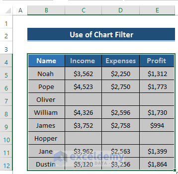
- Select the range of cells B4 to E12.
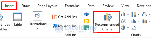
- Go to the Insert tab in the ribbon.
- From the Charts group, select Recommended Charts.
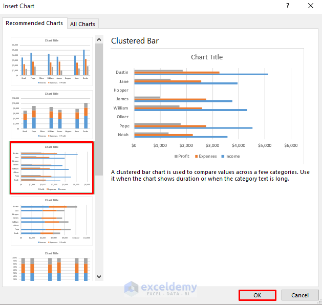
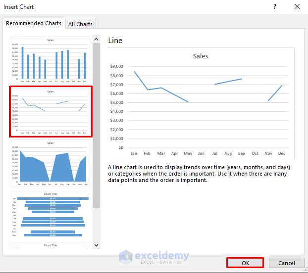
- The Insert Chart option will appear.
- Select the Clustered Bar chart.
- Click on OK.
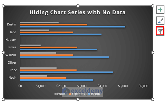
- We have a bar chart. But some of the portions are blank as there are no values in them.
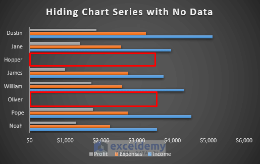
- We need to use a chart filter and remove the blank portions.
- Click on the Chart Filter icon on the right side of the chart.
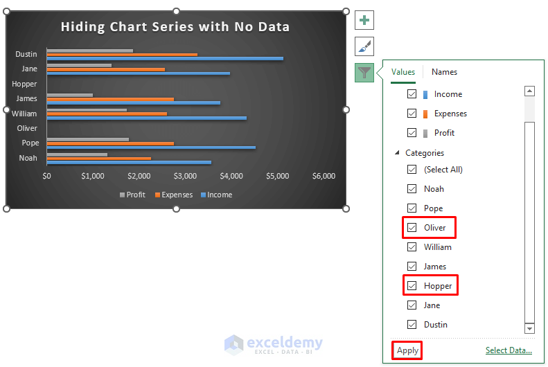
- It will open up several options.
- As we don’t have values for Oliver and Hopper, we need to uncheck them from the Categories section.
- Click on Apply.
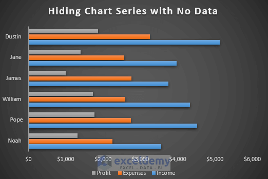
- We will get the result as shown in the image below.
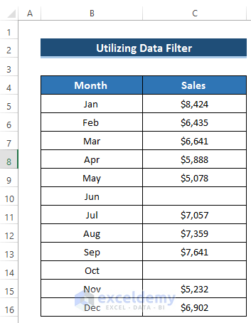
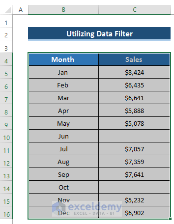
Method 2 – Utilizing Data Filter
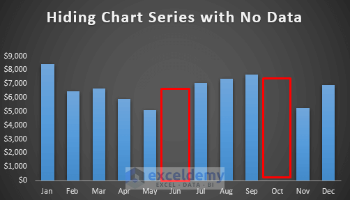
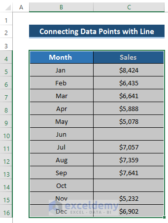
In the dataset, we don’t any sales amounts for the months of June and October.
Steps:
- Select the range of cells B4 to C16.
- Go to the Data tab in the ribbon.
- From the Sort & Filter group, select the Filter option.
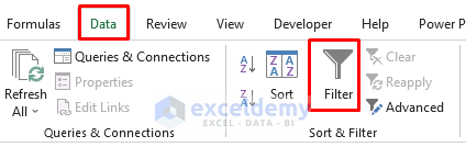
- It will add filter arrows to the dataset.
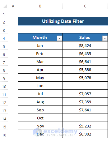
- Go to the Insert tab in the ribbon.
- From the Charts group, select Recommended Charts.
- The Insert Chart option will appear.
- Select the Clustered Column chart.
- Click on OK.
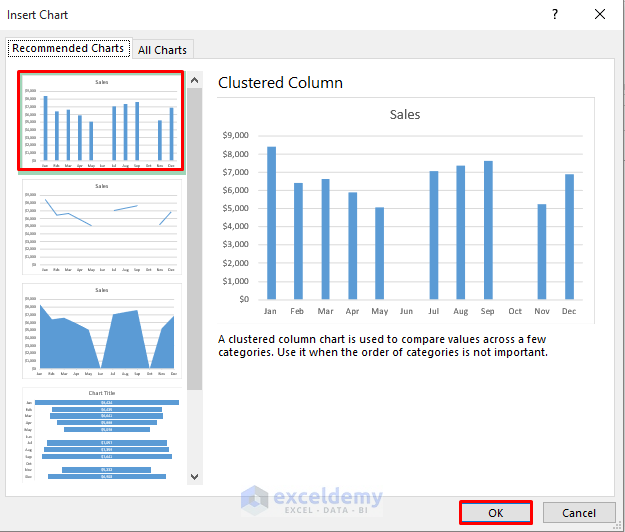
- We have a bar chart. But some of the portions are blank as there are no values in them.
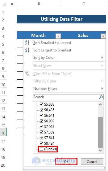
- Go to the dataset and click on the drop-down arrow of the Sales column.
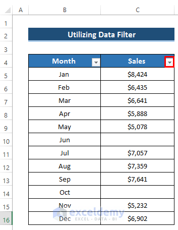
- A new menu will appear.
- Uncheck the Blanks.
- Click on OK.
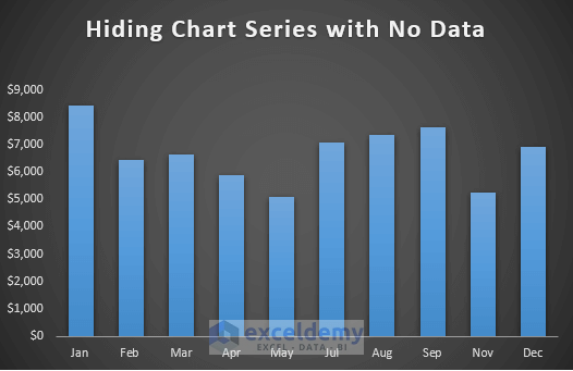
- The result will be as shown in the image below.
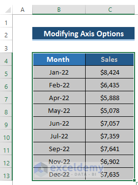
Method 3 – Modifying Axis Options
Steps
- Select the range of cells B4 to C13.
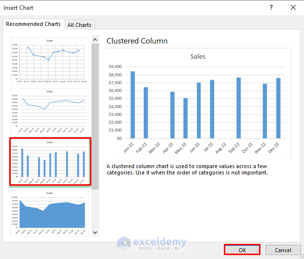
- Go to the Insert tab in the ribbon.
- From the Charts group, select Recommended Charts option.
- The Insert Chart option will appear.
- Select the Clustered Column chart.
- Click on OK.
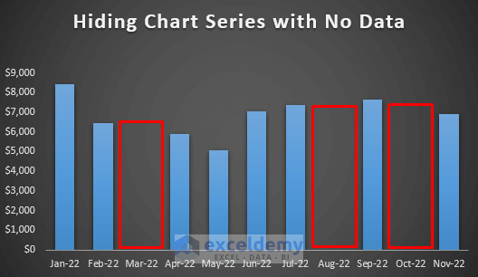
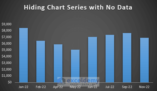
- It will give us the following results where we will see some blank portions.
- This is because we do not have any data in those months.
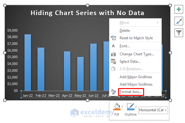
- To hide those blank portions, we need to double-click on the horizontal axis or right-click on the horizontal axis to open the Context Menu.
- Select Format Axis.
- The Format Axis dialog box will open.
- From the Axis Options section, select the Text axis.
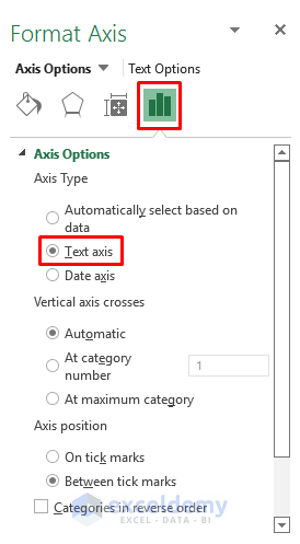
- The result will be as shown in the image below.
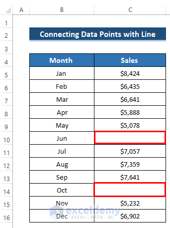
Method 4 – Connecting Data Points with Line
Steps:
- Select the range of cells B4 to C16.
- Go to the Insert tab in the ribbon.
- From the Charts group, select Recommended Charts.
- The Insert Chart option will open.
- Select the Line chart.
- Click on OK.
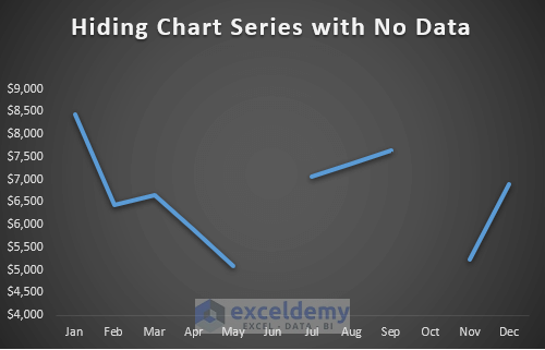
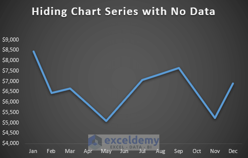
- It will give us the following chart where some of the data are missing.
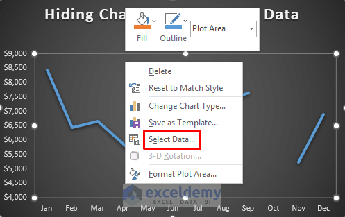
- Right-click on the chart.
- It will open up the Context Menu.
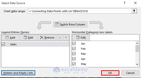
- Click on Select Data.
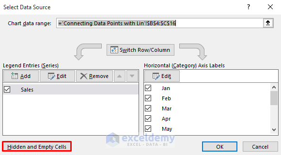
- It will open up the Select Data Source dialog box.
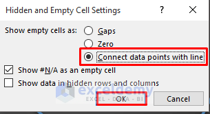
- Select Hidden and Empty Cells.
- The Hidden and Empty Cells Settings dialog box will open.
- Click on the Connect data points with line.
- Click on OK.
- In the Select Data Source dialog box, click on OK.
- We will get the desired chart that hides the series with no data.
Download Practice Workbook
Related Articles
<< Go Back To Data Series in Excel | Excel Charts | Learn Excel
Get FREE Advanced Excel Exercises with Solutions!
