Excel has a large built-in spreadsheet to input data. However, most of the time, many of the cells remain unused. To prevent the entry of any scatter data on the datasheet, we can hide the unused cells in several ways. In this article, we will demonstrate 3 easy methods to hide unused cells in Excel. If you are curious about it, download our practice workbook and follow us.
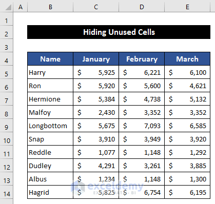
To demonstrate the approaches, we consider a dataset of 10 employees of any organization and their salaries in the first quarter of any year. So, our dataset is in the range of cells B5:E14. We are going to hide the rest of the unused cells in the spreadsheet.
1. Using Context Menu to Hide Unused Cells in Excel
In this method, we will use the Context Menu to hide the unused cells. We are going to hide all the cells except our dataset. The steps of this process are given below:
📌 Steps:
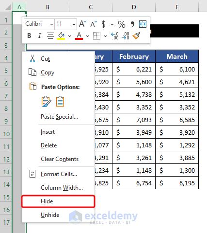
- First, we will hide all the unused columns. For that, select the entire column A.
- After that, right-click on your mouse and choose the Hide option.
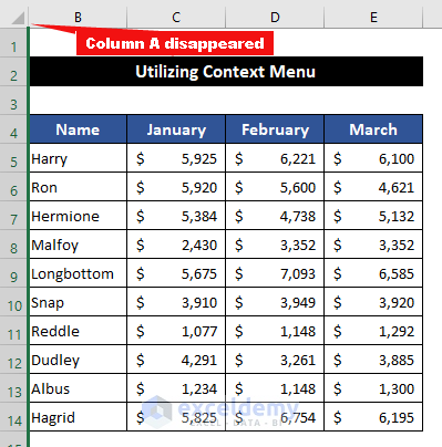
- You will see column A will disappear.
- Similarly, select the entire column F and press ‘Ctrl+Shift+Right Arrow (→)’ to select all the empty columns.
- Again, right-click on your mouse and choose the Hide option.

- All the unused columns will hide from our dataset.

- Now, we are going to hide the unused rows.
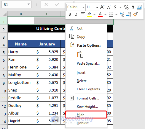
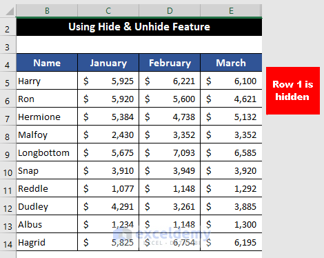
- Select the entire row 1 and right-click on your mouse.
- Then, choose the Hide option.
- Row 1 will disappear.
- Similarly, select the entire row 15 and press ‘Ctrl+Shift+Down Arrow (↓)’ to select all the empty rows.
- Again, right-click on your mouse and choose the Hide option.

- At last. you will get all the unused cells hidden from our spreadsheet.
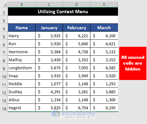
Thus, we can say that our method worked perfectly, and we are able to hide unused cells in Excel.
Read More: How to Hide Extra Cells in Excel
2. Applying Excel Hide & Unhide Feature to Hide Unused Cells
In this process, we are going to use the Hide & Unhide feature from the drop-down of the Format command to hide the unused cells. We will hide all the cells except our dataset. The steps of this approach are given as follows:
📌 Steps:
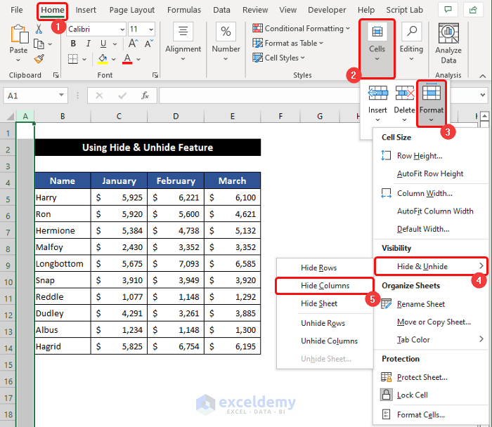
- At first, we are going to hide all the unused columns. For that, select the entire column A.
- Then, in the Home tab, click the drop-down arrow of the Format option and choose the Hide Columns option from the Hide & Unhide Menu, located in the Cells group.
- You will see column A will disappear.

- Again, select the entire column F and press ‘Ctrl+Shift+Right Arrow (→)’ to select all the empty columns.
- Similarly, click the drop-down arrow of the Format option and choose the Hide Columns option from the Hide & Unhide Menu, located in the Cells option.

- All the unused columns will hide from our dataset.
- Now, we will hide the unused rows.
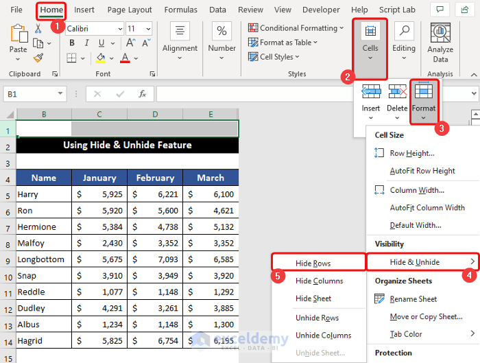
- For doing that, select the entire row 1.
- Afterward, in the Home tab, click the drop-down arrow of the Format option and choose the Hide Rows option from the Hide & Unhide Menu, located in the Cells group.
- Row 1 will disappear.
- Similarly, select the entire row 15 and press ‘Ctrl+Shift+Down Arrow (↓)’ to select all the empty rows.
- Then, click the drop-down arrow of the Format option and choose the Hide Columns option from the Hide & Unhide Menu, located in the Cells group.

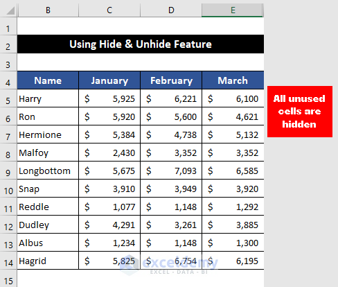
- Finally, you will notice all the unused cells hidden from our spreadsheet.
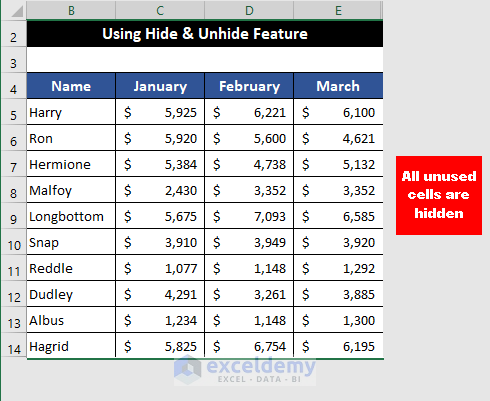
So, we can say that our method worked effectively, and we are able to hide unused cells in Excel.
Read More: How to Hide Blank Cells in Excel
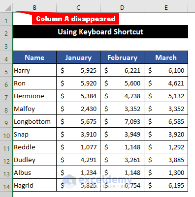
3. Using Keyboard Shortcut to Hide Unused Cells in Excel
In this approach, we will use the keyboard shortcut to hide the unused cells. The procedure of this method is shown below:
📌 Steps:
- First, we will hide all the unused columns. For that, select the entire column A.

- Afterward, press ‘Ctrl+0’ to hide the column.
- You will see column A will disappear.
- Similarly, select the entire column F and press ‘Ctrl+Shift+Right Arrow (→)’ to select all the empty columns.
- Again, press ‘Ctrl+0’, and all the unused columns will hide from our dataset.
- Now, we will hide the unused rows.
- For that, select the entire row 1.
- Then, press ‘Ctrl+9’, and you will notice row 1 will disappear.

- Similarly, select the entire row 15 and press ‘Ctrl+Shift+Down Arrow (↓)’ to select all the empty rows.
- Again, press ‘Ctrl+9’ on your keyboard.
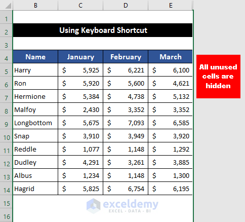
- In the end, you will get all the unused cells hidden from our spreadsheet.

Finally, we can say that our method worked successfully, and we are able to hide unused cells in Excel.
Download Practice Workbook
Download this practice workbook for practice while you are reading this article.
Conclusion
That’s the end of this article. I hope that this article will be helpful for you and you will be able to hide unused cells in Excel. Please share any further queries or recommendations with us in the comments section below if you have any further questions or recommendations. Keep learning new methods and keep growing!
Related Articles
- Hide Data in Excel
- How to Hide Cells in Excel Until Data Entered
- How to Hide Part of Text in Excel Cells
- How to Hide Confidential Data in Excel
- How to Hide Highlighted Cells in Excel
<< Go Back to Hide Cells | Excel Cells | Learn Excel
Get FREE Advanced Excel Exercises with Solutions!
