In this article, we will discuss how to hide cells in Excel until data is entered.
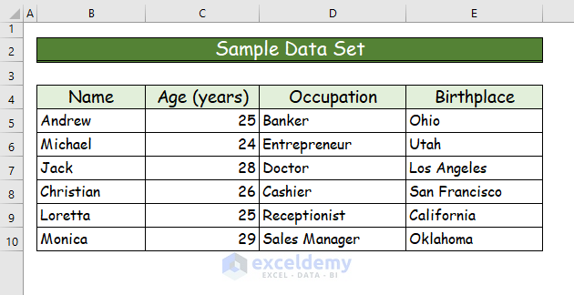
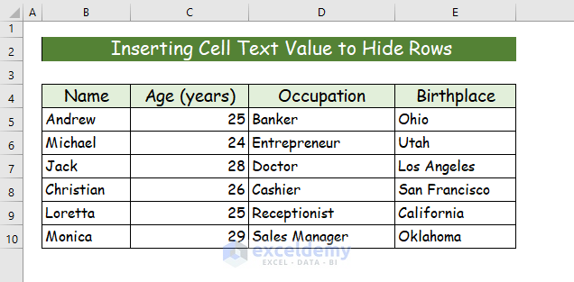
We will use the dataset below, which contains some numeric and some text values, to demonstrate two different methods to hide cells until data is entered. In the first procedure, we will change the cell format of some particular cells, and in the second we will apply VBA code to hide rows and columns of the dataset respectively.
Method 1 – Changing Cell Format to Hide Cells in Excel Until Data Is Entered
Steps:
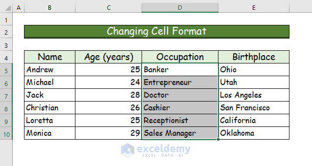
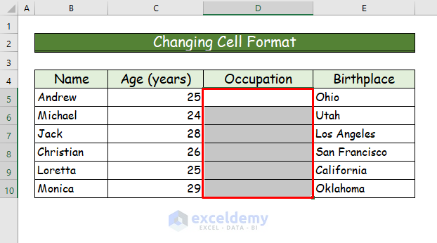
- Select the cells to hide.
- Right-click on the cells after selecting them and choose the Format Cells… command from the context menu.
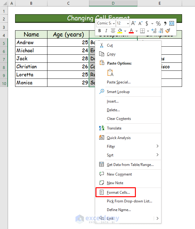
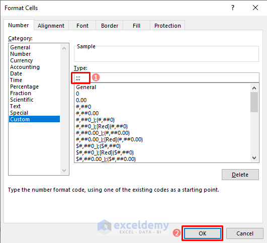
A dialog box named Format Cells opens.
- Choose the Custom command under the Number tab.
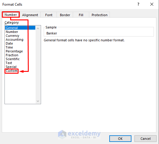
- Type three semicolons (;) in the Type box.
- Click OK.
The selected cells in the dataset will be empty.
To unhide the cells:
- Select the Format Cells… command again.
- Choose the original number format of the data. Here, the Text format.
- Click OK.
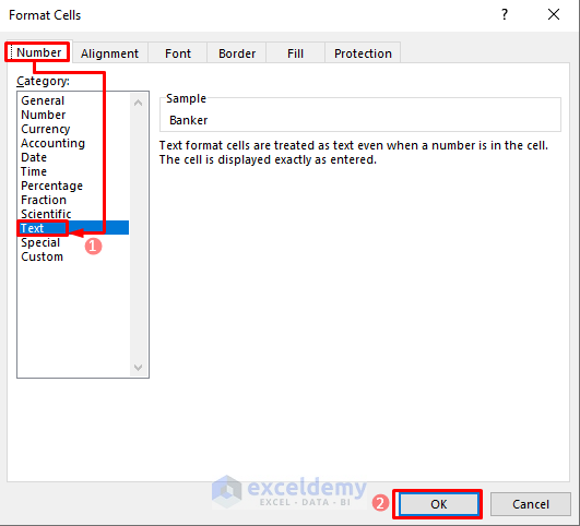
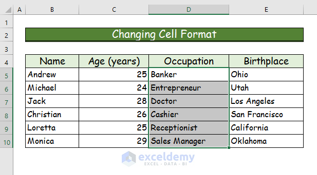
The data will be visible in the cells again.
Method 2 – Applying VBA to Hide Cells in Excel
In our previous approach, we hid some cells in our data set by changing the cell format. Now, we will apply VBA to hide an entire row or column based on its cell values.
2.1 – Inserting a Cell Text Value to Hide Rows Automatically
To hide an entire row, we will specify a text value from the dataset in the code.
Steps:
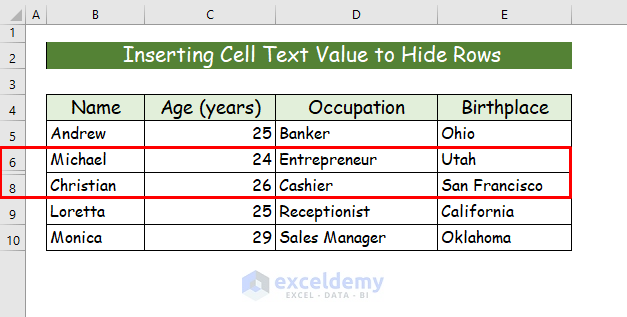
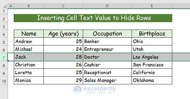
We’ll apply our code to the following dataset.
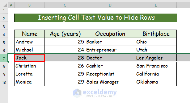
- Choose any specific text value from any cell. For example, the name Jack, which is in row 7.
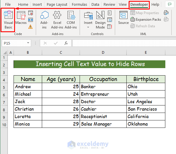
- Choose the Visual Basic command from the Developer tab of the ribbon.
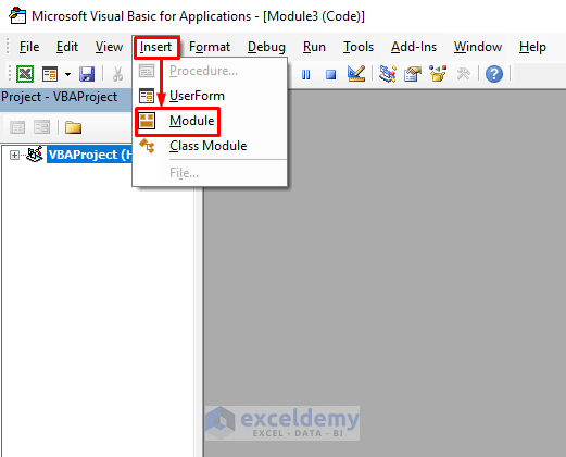
- Choose the Module command from the Insert tab in the pop-up window.
- Copy the following code and paste it into the module window that opens:
'Set the name of the function
Sub Inserting_Text_Value_to_Hide_Row()
'Declaring the first row of the data set
StartRow = 4
'Declaring the last row of the data set
LastRow = 10
'Addressing the column number that holds the text value
iCol = 2
'Finding the specific word of the above from first row to last row of the data set and hide the row
For i = StartRow To LastRow
'Start to find the specific word Jack from the adressed row by looping. If the word is not found, then the rows wont'be hidden
If Cells(i, iCol).Value <> "Jack" Then
Cells(i, iCol).EntireRow.Hidden = False
'If the word is found in the specific column then the rows will be hidden
Else
Cells(i, iCol).EntireRow.Hidden = True
End If
Next i
End Sub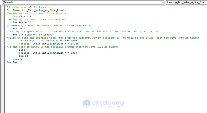
➤ We define the function name of the VBA as Inserting_Text_Value_to_Hide_Row.
➤ We set the first row with StartRow= 4 since our dataset starts in row 4.
➤ We set the last row of the data set with LastRow=10 as our last data is in row 10.
➤ We give the number of the column in which the text value is located with iCol=2.
➤ With the IF fucntion, we look for the word “Jack” sequentially from the addressed first row (4) to the last row (10) of the dataset. If the loop variable i finds the word “Jack” in any row of the declared column (B), then it hides the entire row from the dataset automatically. It continues to loop until it has searched in all the rows.
➤ Finally, the ELSE function ensures that if the specific word is not found, then no row will be hidden.
- Save the code and press the Play button to run it.
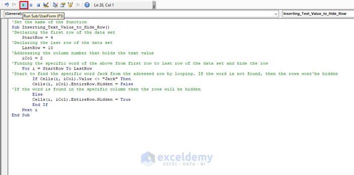
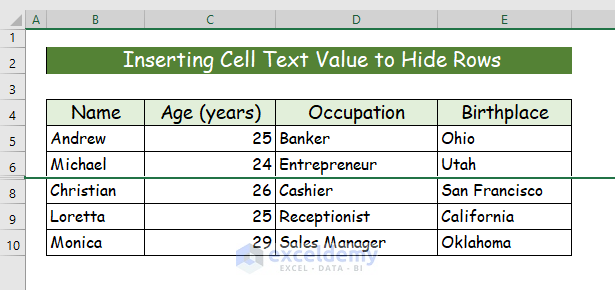
Row 7, containing the word Jack, is hidden.
- To show the specific row again, click between rows 6 and 8.
- Right-click on the selection and choose the Unhide command from the context menu.
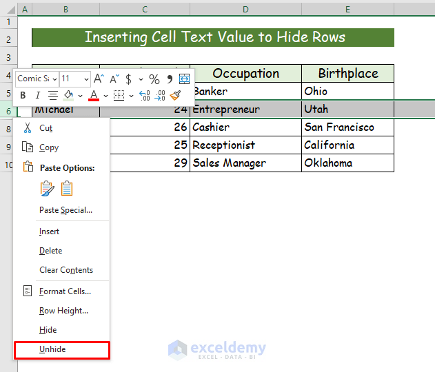
The row is visible again.
2.2 – Inserting a Cell Numeric Value to Hide Columns Automatically
We can also hide an entire column based on a cell value by applying VBA, similarly to the previous method. In this approach, we will insert a numeric value from the dataset into the code to hide the column.
Steps:
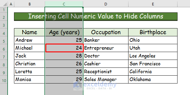
- Select a random numerical value from the data set. For our working purpose, we will take the numerical value 24 in column C.
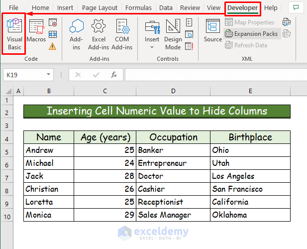
- Go to the Developer tab and choose the Visual Basic command.
- Select Insert, then Module.
- Copy the following code and paste it into the Module window like in the previous procedure:
'Address the function name
Sub Inserting_Numeric_Value_to_Hide_Column()
'Declare the first column, last column and the row number that holds the numeric value in the data set
StartColumn = 2
LastColumn = 5
iRow = 7
'Finding the specific number from first column to last column of the data set and hide the column
For i = StartColumn To LastColumn
If Cells(iRow, i).Value <> "24" Then
Cells(iRow, i).EntireColumn.Hidden = False
Else
Cells(iRow, i).EntireColumn.Hidden = True
End If
Next i
End Sub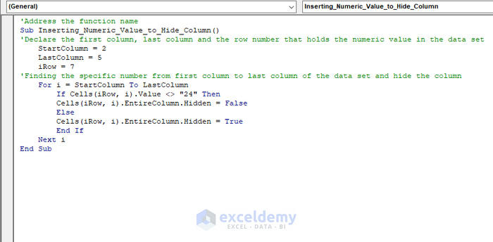
➤ We name the function Inserting_Numeric_Value_to_Hide_Column.
➤ We set the first column with StartColumn= 2 sinceour dataset starts in column 2.
➤ We set the last row of the dataset with LastColumn= 5.
➤ We provide the number of the row in which the numeric value is located with iRow=7.
➤ With the IF function, we look for the number “24” from the addressed first column (2) to the last column (5) of the data set. If the loop variable i finds the number “24” in any column of the declared row (7), it hides the entire column from the data set automatically. It continues to loop until it has searched in all the columns.
➤ Finally, with the ELSE function, if the specific number is not found, then no column will be hidden.
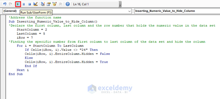
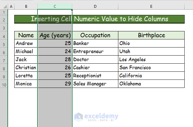
- Save the code and press F5 or the Play button to run it.
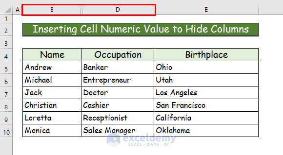
Column C is hidden from the dataset.
- To unhide the column, click in between columns C and D.
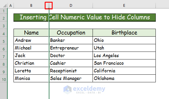
- Right-click on the selection and choose the Unhide command from the context menu.
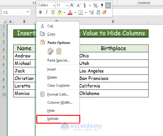
The column will be visible in the data set again.
Read More: How to Hide Extra Cells in Excel
Download Practice Workbook
You can download the free Excel workbook here and practice on your own.
Related Articles
- Hide Data in Excel
- How to Hide Confidential Data in Excel
- How to Hide Highlighted Cells in Excel
- How to Hide Part of Text in Excel Cells
- How to Hide Unused Cells in Excel
- How to Hide Blank Cells in Excel
<< Go Back to Hide Cells | Excel Cells | Learn Excel
Get FREE Advanced Excel Exercises with Solutions!
