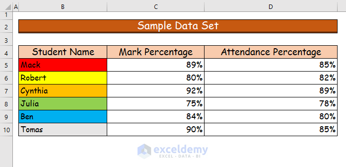
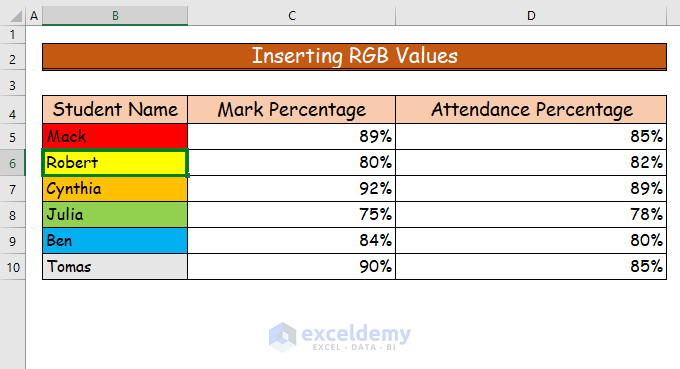
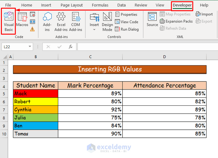
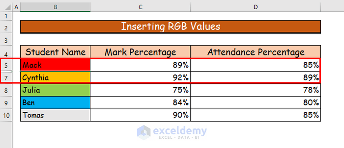
How to Hide Highlighted Cells in Excel (2 Ways)

We will use the following data set. We have some student names, their grade percentages, and their attendance percentages. In the Student Name column, we have highlighted each cell in different colors. We will hide those cells.

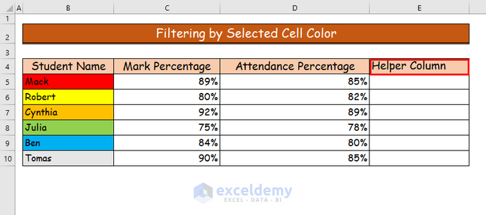
Method 1 – Filtering by Selected Cell Color to Hide Highlighted Cells in Excel

Steps:

Create a helper column in column E.

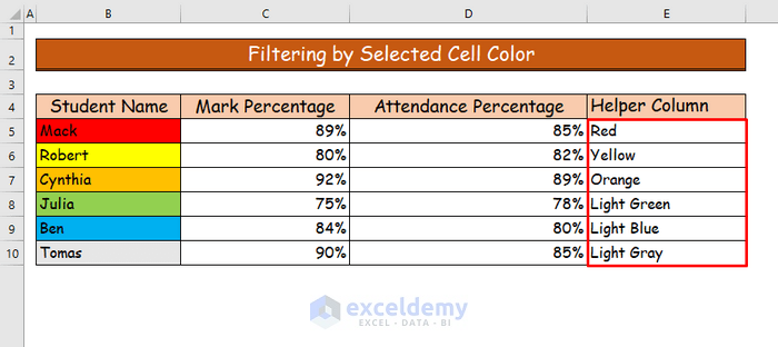
Write down the colors of each cell from column B in the helper column.

Select the whole helper column and then go to the Data tab of the ribbon.
Go to the Filter command under the Sort & Filter group.

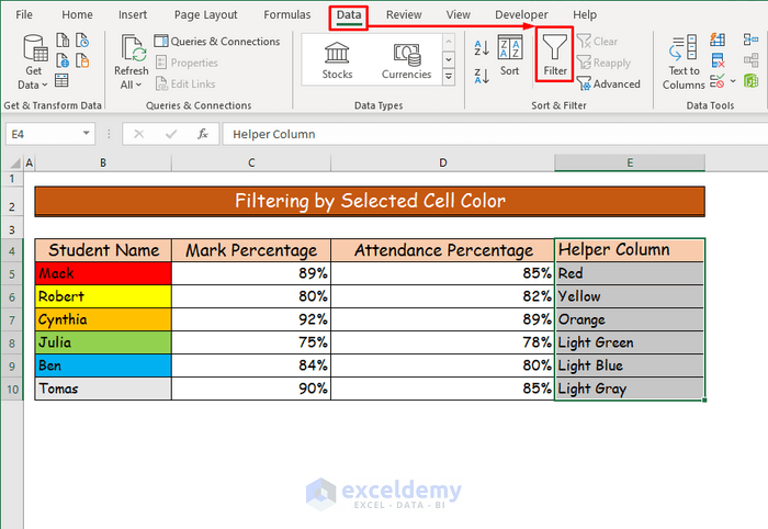
This command will allow you to filter the data range from B4:B10 based on their color.
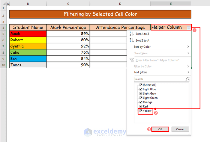
Press the drop-down button in the helper column.
You will see all the filter options from the drop-down.
Under the Select All command, you will notice all the cell colors as options in there.
Unmark any cell color, and after unmarking, you will not see the cell in the data set. We will choose the color Yellow.

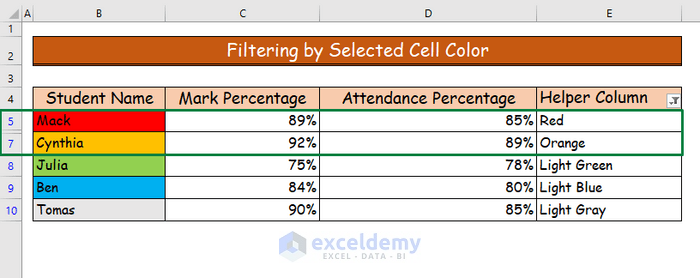
Here’s the filtered result.

If you want to show the hidden cell, go to the filter drop-down again and check a specific cell color.

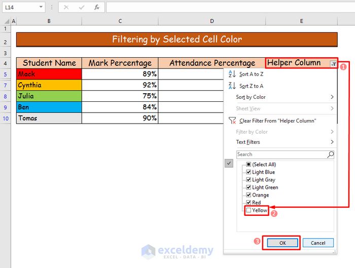
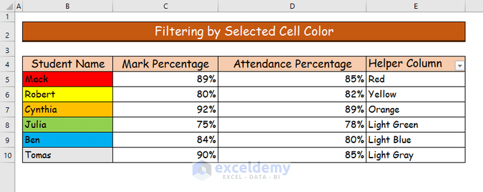
You will see the highlighted cell with its corresponding row again.

Method 2 – Applying VBA to Hide Highlighted Cells in Excel

Case 2.1 – Inserting RGB Values

Steps:

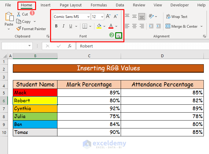
Select any highlighted cell from column B to determine its RGB value. We will find out the RGB value of the color yellow which is in cell B6.

Go to the Home tab of the ribbon.
Choose the little arrow on the lower-right corner of the Font group.

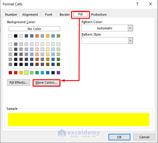
A dialog box named Format Cells will appear.
Go to the Fill tab.
Choose More Colors….

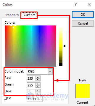
Another dialog box named Colors will appear.
Go to the Custom tab and you will find the RGB value for yellow which is 255,255,0.

Go to the Developer tab in the ribbon and select the Visual Basic command.

You will see the VBA window.
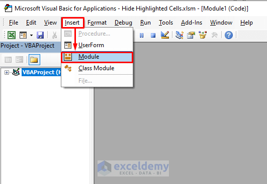
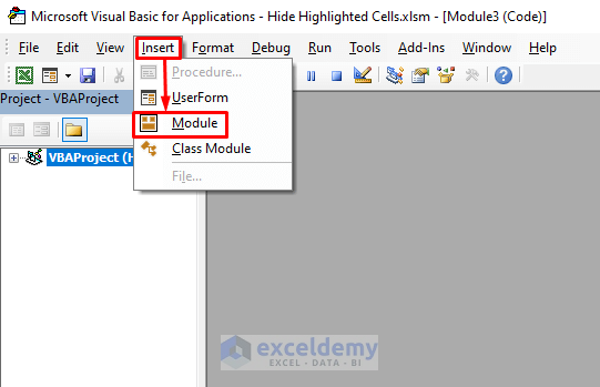
Choose the Module command from the Insert tab.

Copy the following VBA code into the module.

'Set the function name
Sub Hide_Rows_by_Inserting_RGB_Values()
'Declare the row till which the data remains
Dim EndRow As Long
'Declare the counter variable
Dim y As Long
'Set the rows property and count all the available rows
'Set the column number in which the highlighted cell is
EndRow = Cells(Rows.Count, 2).End(xlUp).Row
'Scan each row in column B and check the cell is yellow by for looping
For y = 4 To EndRow
'Set the cells property and looking for interior color throguh RGB function
If Cells(y, 2).Interior.Color = RGB(255, 255, 0) Then
'Set what happens after the condition is met
Rows(y).Hidden = True
'End the If function
End If
'Repeat the steps to complete until last row appears
Next y
End Sub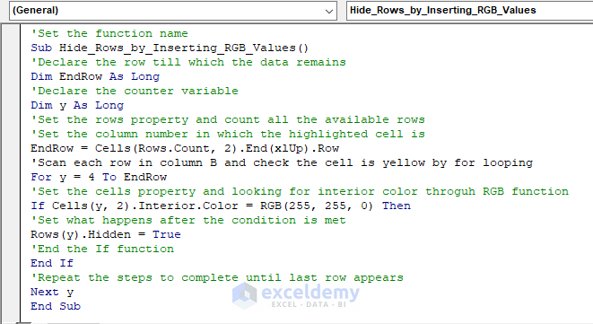

VBA Code Breakdown

The function name is Hide_Rows_by_Inserting_RGB_Values.
The variable names are EndRow and y and they are long type variables.
EndRow = Cells(Rows.Count, 2).End(xlUp).Row: We set the row property and count all available rows and also set the column number in which the highlighted cell is.
For y = 4 To EndRow: We will use this for looping to check each row in column B staring from cell B4 to find the yellow cell color.
If Cells(y, 2).Interior.Color = RGB(255, 255, 0)Rows(y).Hidden = True: With the IF function we will look for the color according to their RGB value which is 255,255,0 for yellow. If the condition is met then this code will hide the entire row.
End If: The end of the IF function.
Next y: We will continue to look through the last row to meet the condition.

Save the file as .xlsm and press the play button or F5 to run the code.

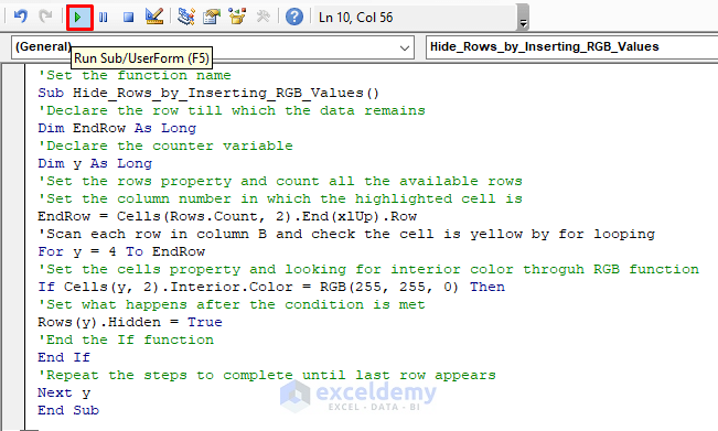
The B6 cell containing the yellow color has been hidden from the data table.

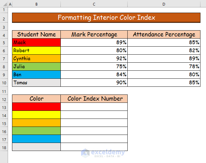
Case 2.2 – Formatting by the Interior Color Index

Steps:

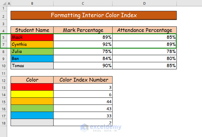
We have to create another data table under the main data set where we will find out the color index number of the highlighted cells.

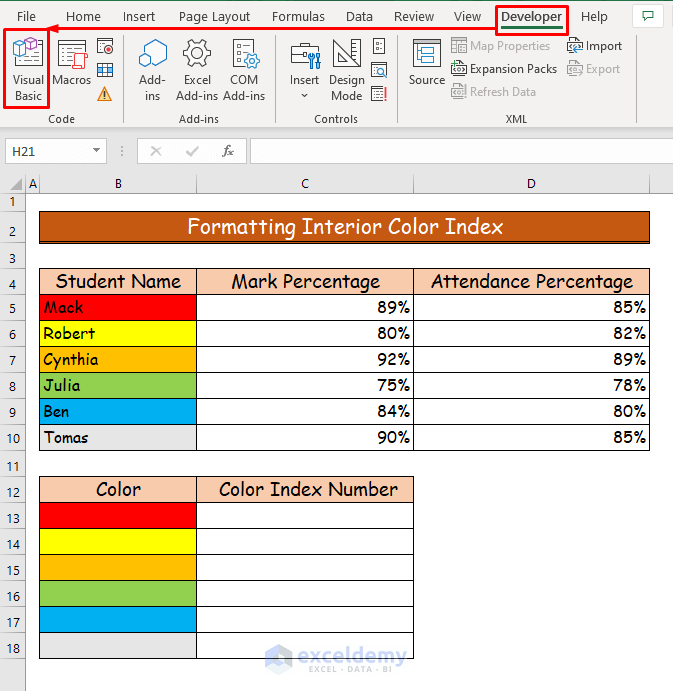
Go to the Visual Basic command from the Developer tab in the ribbon.

Go to the Module command from the Insert tab.

Paste in the following code and save.

'Set the function name
Function GetColorIndex(VarRange As Range) As Integer
'Set code to get color index number
GetColorIndex = VarRange.Interior.ColorIndex
End Function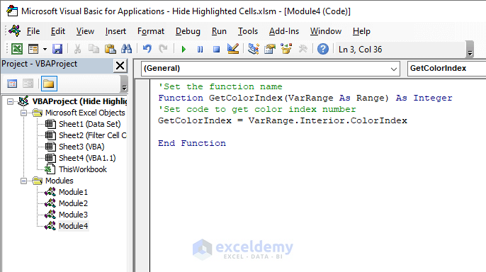

In the worksheet, use the following formula in cell C13 to get the color index number for its corresponding cell’s color.

=GetColorIndex(B13)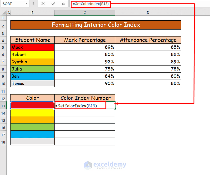

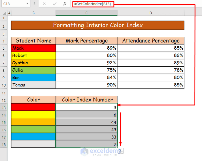
Press Enter and use the AutoFill feature to drag the formula to the lower cells. You will be able to find out the color index numbers for all the colors.

Go to the VBA window again and paste the following code.

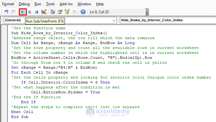
'Set the function name
Sub Hide_Rows_by_Interior_Color_Index()
'Address range object, the row till which the data remains
Dim Cell As Range, cRange As Range, EndRow As Long
'Set the rows property and count all the available rows in current worksheet
'Set the column number in which the highlighted cell is in current worksheet
EndRow = ActiveSheet.Cells(Rows.Count, "B").End(xlUp).Row
'Go through from row 4 in column B and check the cell is yellow
Set cRange = Range("B4:B" & EndRow)
For Each Cell In cRange
'Set the cells property and looking for interior color throguh color index number
If Cell.Interior.ColorIndex = 6 Then
'Set what happens after the condition is met
Cell.EntireRow.Hidden = True
'End the If function
End If
'Repeat the steps to complete until last row appears
Next Cell
End Sub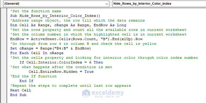

VBA Code Breakdown

The function name is Hide_Rows_by_Interiror_Color_Index.
The variable names are Cell , cRange which are range type variables, and the last one is EndRow which is long type variable.
EndRow = ActiveSheet.Cells(Rows.Count, “B”).End(xlUp).Row: We set the row property and count all available rows and also set the column number in which the highlighted cell is.
Set cRange = Range(“B4:B” & EndRow): We will use this to go through each row in column B from cell B4 till the last row.
If Cell.Interior.ColorIndex = 6 Then Cell.EntireRow.Hidden = True: With the IF function, we will look for the color according to their color index number from the data set which is 6 for yellow. If the condition is met then this code will hide the entire row.
End If: The end of the IF function.
Next Cell: We will continue to look through the last row to meet the conditions.