How to Hide a Part of Text in Excel Cells (2 Methods)

Dataset Overview

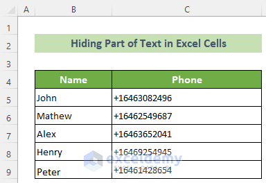
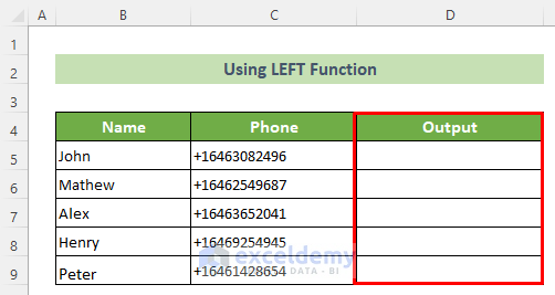
Let’s assume we have a dataset of 5 employees’ phone numbers. But we don’t want to show it to everyone. So, we need to hide some part of the text of the phone number cells. You can accomplish this result using any of the following methods.

Method 1 – Custom Format

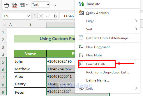
Select the dataset (e.g., cells C5 to C9) where you want to hide parts of text.
Right-click and choose Format Cells.

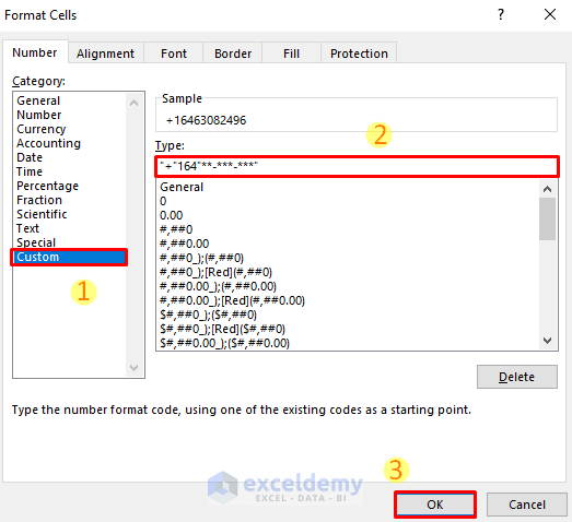
In the Format Cells window, select Custom from the Category pane.
In the Type box, enter the format:

"+"164"**-***-***"

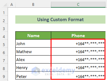
Click OK to hide the phone numbers while maintaining a certain sequence.

Method 2 – Excel Functions

2.1 Hide Right Part of Text Using LEFT Function

Create a new column (e.g., Output) to apply formulas.

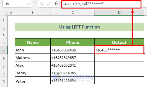
For the first 6 digits of the phone number, enter the following formula in cell D5:

=LEFT(C5,6)&"******"

Press Enter.
As a result, you will get the phone number with the first 6 digits and the rest hidden as star (*) marks.

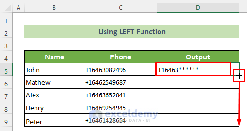
Drag the formula down to apply it to other cells.

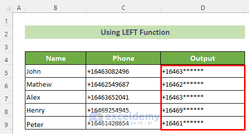
As a result, you will get all your employees’ phone numbers with some hidden parts. The output will look like this.

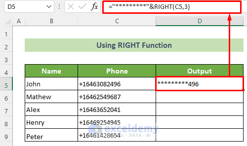
2.2 Hide Left Part of Text Using RIGHT Function

To show only the last 3 digits:

Click on cell D5.
Enter the following formula in the formula bar:

="*********"&RIGHT(C5,3)

Press Enter.

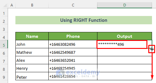
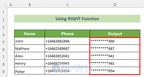
Drag the formula down to apply it to other cells.

The first part of the phone number is hidden and only the last 3 digits are visible for each employee’s phone number.

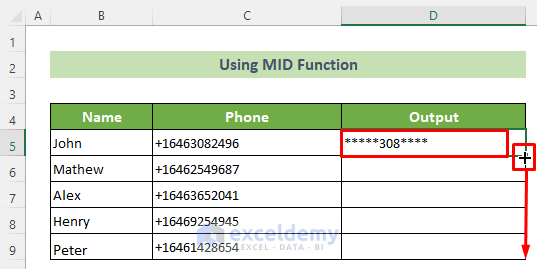
2.3 Hide Left & Right Part of Text Using MID Function

To only show the middle digits:

Click on the D5 cell.
Enter the following formula in the formula bar.

="*****"&MID(C5,6,3)&"****"

Press Enter.

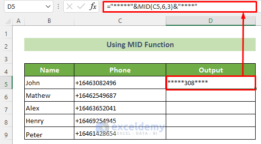
The first and last part of the cell value have been hidden and only 3 digits from the middle is showing.
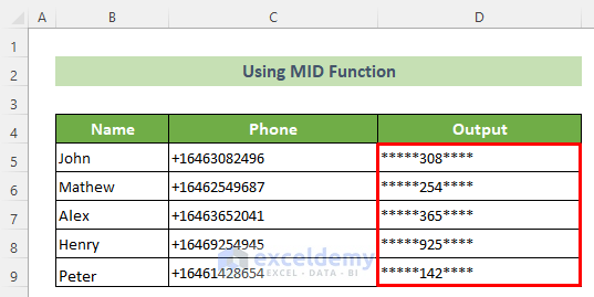
Drag the formula down to apply it to other cells.

The first and last parts of all the phone numbers for all employees have been hidden.

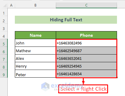
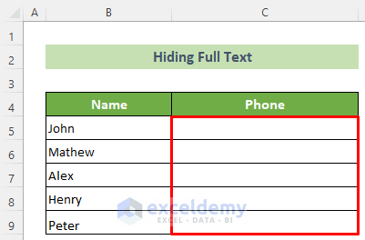
How to Hide Full Text in Excel Cells

Choose the range of cells you want to hide (for example, C5 to C9).
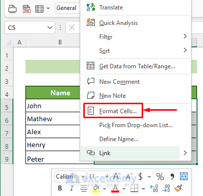
Right-click on the selected cells.

From the Context Menu, choose Format Cells.

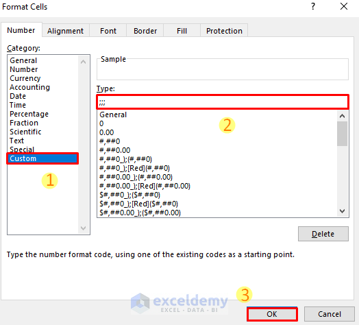
In the Format Cells dialog box, select the Custom option from the Category pane.
In the Type box, enter three consecutive semicolons (;;;).
Click OK.

The full text of the cells will be hidden. The values remain in the cell but are not displayed. For example, the result will look like this: