Sometimes for data visualization, you may need to create a floating bar chart in Excel. So, if you are looking for how to make this chart in Excel, then you have come to the right place. Today, in this article, I will create this chart using Excel’s Microsoft 365 version.
Floating Bar Chart in Excel: 2 Suitable Methods
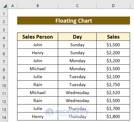
Here, I will demonstrate 2 suitable methods for making a floating bar chart in Excel. For your better understanding, I will use a sample dataset. Which has 3 columns. They are Sales Person, Day, and Sales. The dataset is given below.
1. Use of Line Chart for Making Floating Bar Chart in Excel
Here, I will demonstrate 3 easy steps for making a floating bar chart in Excel. Later, I will show you how to make a floating column chart in Excel. Now, you may see the following steps for creating the floating bar chart.
Step 1: Removing Duplicate Values
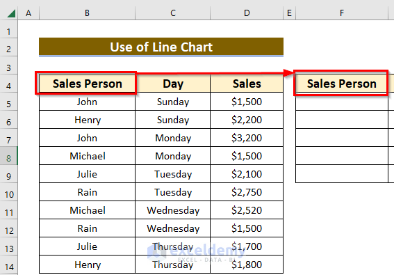
Here is the first step. Basically, to make the floating bar chart, firstly, you have to find all the unique values that will act as X-values (abscissa of the coordinate).
- First, write down the particular column header of the criteria range. Here, I have written Sales Person in the F4 cell as the column header of criteria.
- Then, open the Advanced Filter option by clicking the Data tab >> Sort & Filter >> Advanced.

As a result, you will see a new dialog box named Advanced Filter.
- First, mark Copy to another location.
- Later, specify the range (‘Floating Chart’!$B$4:$D$14) in the List range option. Here, the ‘Floating Chart’ is the name of the worksheet.
- Then, provide the criteria (‘Floating Chart’!$B$4:$B$14) in the Criteria range box.
- After that, choose the space (‘Floating Chart’!$F$4:$F$14) in the Copy to box. Here, you must select enough space.
- Then, mark Unique records only.
- Subsequently, press OK.

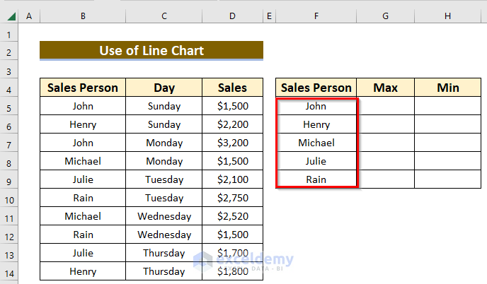
- Finally, you’ll see the following output.
Read More: How to Flip Bar Chart in Excel
Step 2: Required Calculations for Floating Bar Chart
Now, I need to do some calculations for making the floating bar chart in Excel. In this case, I’m going to use two functions. They are MAXIFS and MINIFS functions.
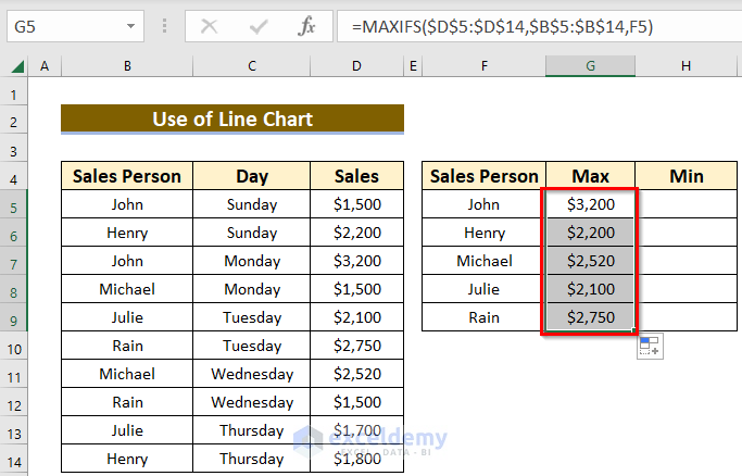
- Firstly, write the following formula in the G5 cell.
=MAXIFS($D$5:$D$14,$B$5:$B$14,F5)Here, in this formula, $D$5:$D$14 is the range for maximum value, $B$5:$B$14 is the criteria range, and F5 is the criteria for which this function will find the maximum value.
- Secondly, press ENTER.
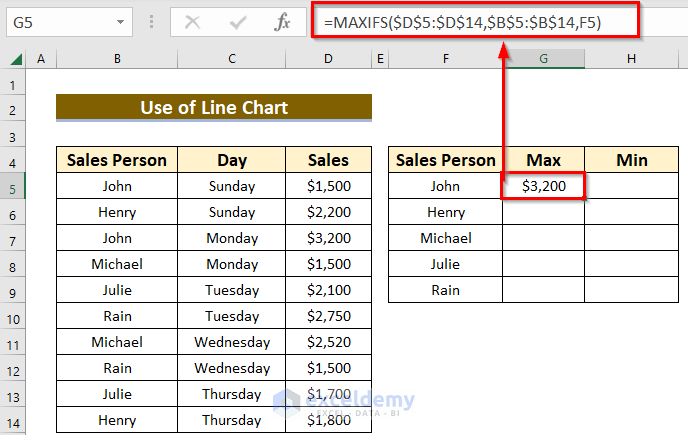
- Now, use the Fill Handle icon to paste the used formula to the other cells of the column.

As a result, you will find all the maximum values for all the salespeople.
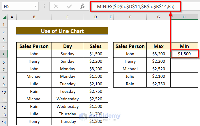
- Similarly, write the following formula in the H5 cell.
=MINIFS($D$5:$D$14,$B$5:$B$14,F5)Here, in this formula, $D$5:$D$14 is the range for minimum value, $B$5:$B$14 is the criteria range, and F5 is the criteria for which this function will find the minimum value.
- Then, press ENTER.
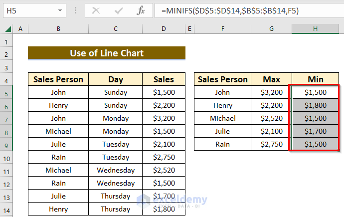
- After that, drag the Fill Handle icon to paste the used formula to the other cells of the column and you will find all the minimum values for the salesperson.
Read More: How to Create a 3D Bar Chart in Excel
Step 3: Inserting Line Chart
Actually, there is a built-in process in Excel for making charts under the Charts group feature. In addition, you can use the Line Chart feature to make a floating bar chart in Excel.
- Firstly, you have to select the data. Here, I have selected the range F5:H9.
- Secondly, you have to go Insert tab.
- Thirdly, from the Charts group section >> you have to choose Insert Line or Area Chart >> then from 2-D Line >> Line.
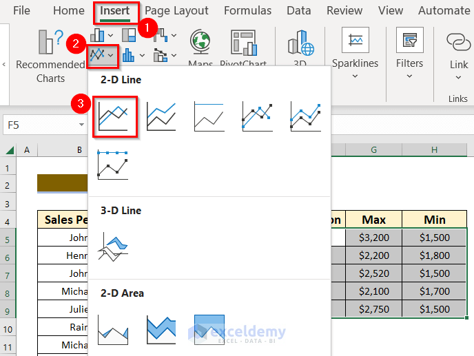
Now, you will see the result.

- Firstly, select the chart >> then from the Chart Elements >> mark on Up/Down Bars.

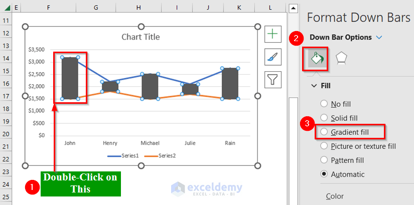
- Then, double-click on the Up/Down Bars.
As a result, you will see a new window named Format Down Bars at the right-most corner of the sheet.
- Now, from the Down Bar Option >> choose Fill & Line >> select Gradient fill.
- Consequently, double-click on Series 1.
As a result, you will see another window named Format Data Series at the right-most corner of the sheet.
- Then, from Series Option >> choose Fill & Line >> select No line.
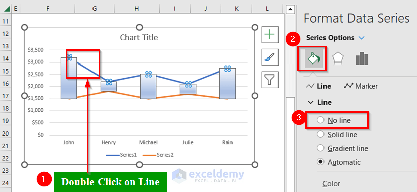
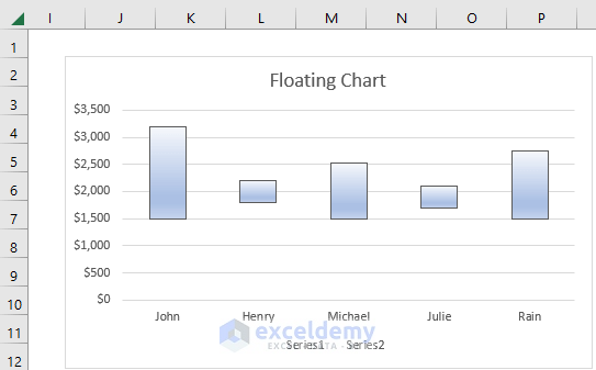
- Similarly, remove the line for Series 2 and you will see the floating bar chart. Here, I have changed the chart title.
Read More: Excel Bar Chart with Line Overlay
2. Utilizing Stacked Column Chart for Creating Floating Bar Chart in Excel
In this section, I will create a floating column chart in Excel. Here, I will use the same dataset. Actually, this is a similar process to the previous one. So, firstly, follow step-1, and step-2 of the previous one to get the unique Sales Person, maximum, and minimum values. Then, follow the steps given below.
Steps:
- Then, write the following formula in the I5 cell.
=G5-H5Here, in this formula, I have found the difference between the maximum and minimum values.
- Subsequently, press ENTER.
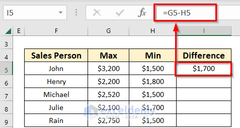
- After that, drag the Fill Handle icon to paste the used formula to the other cells of the column and you will find all the differences between maximum and minimum values.

- After that, you have to select the particular data by pressing the CTRL button. Here, I have selected the range F5, H5:I9.
- Secondly, you have to go Insert tab.
- Thirdly, from the Charts group section >> you have to choose Insert Column or Bar Chart >> then from 2-D Column >> Stacked Column.

As a result, you will see the following chart.

- Consequently, double-click on Series 1.
As a result, you will see a window named Format Data Series at the right-most corner of the sheet.
- Then, from Series Option >> choose Fill & Line >> select No line.

Finally, you will see the floating column chart.
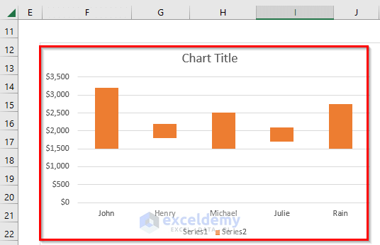
- Here, I have changed the chart title.

Read More: How to Create Overlapping Bar Chart in Excel
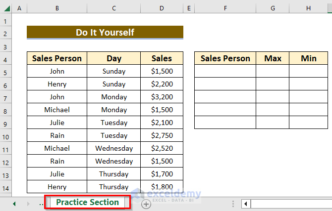
Practice Section
Now, you can practice the explained method by yourself.
Download Practice Workbook
You can download the practice workbook from here:
Conclusion
I hope you found this article helpful. Here, I have described how to make a Floating Bar Chart in Excel. Please, drop comments, suggestions, or queries if you have any in the comment section below.
Related Articles
- How to Show Variance in Excel Bar Chart
- How to Create a Bar Chart with Standard Deviation in Excel
- How to Create a Radial Bar Chart in Excel
- How to Create Construction Bar Chart in Excel
- How to Create Butterfly Chart in Excel
<< Go Back to Create a Bar Chart in Excel | Excel Bar Chart | Excel Charts | Learn Excel
Get FREE Advanced Excel Exercises with Solutions!
