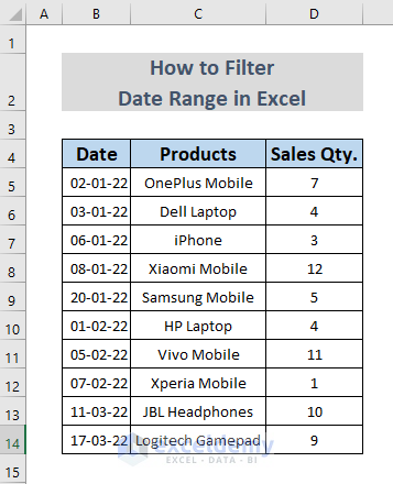
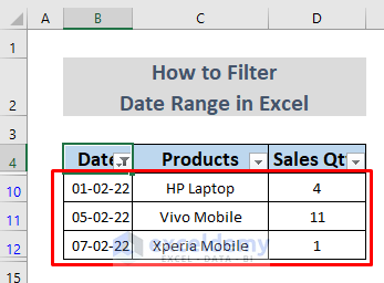
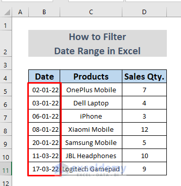
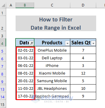
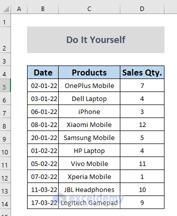
We’ll consider the sample dataset that contains the sales quantity of some electronic products in a shop in January, February, and March. We’ll filter the sales based on a date range.
Method 1 – Using the Excel Filter Command to Filter a Date Range
Case 1.1 – Filtering a Date Range by Selection
We’ll get the sales quantity in the months of January and March.
Steps:
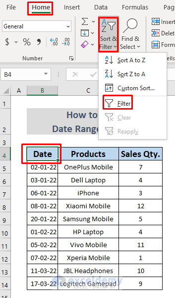
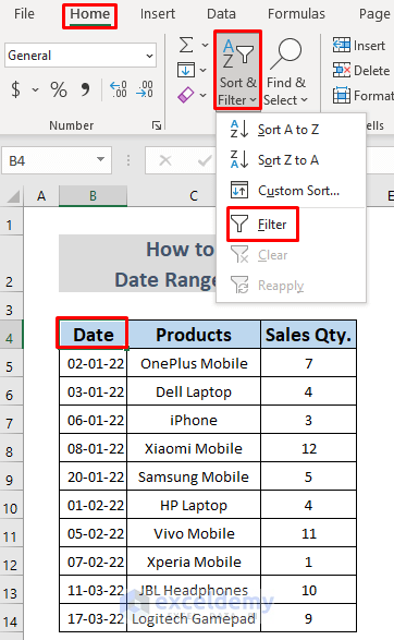
- Select cell B4.
- Go to Home, then to Sort & Filter, and select Filter.
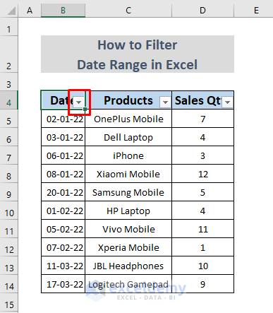
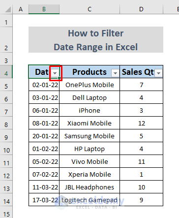
- Click on the drop-down icon in cell B4.
- Unmark January and March and click OK.
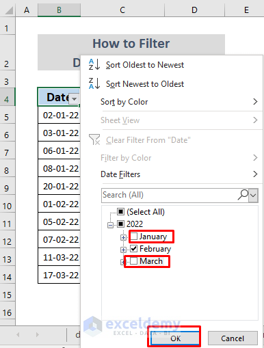
- You will see the information about the sales in February.
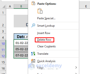
- Select the range B10:D12 and right-click on any of the selected cells.
- Click on Delete Row.
- A warning message will appear. Click OK.
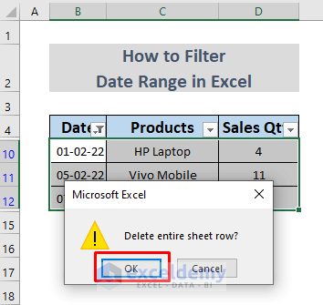
- This operation will remove all the information of the product sales in February.
- Select Filter from Sort & Filter ribbon again.
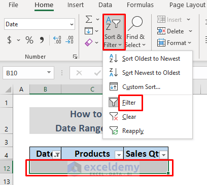
- You will see the information about the sales in January and March only.
Case 1.2 – Filtering a Date Range Using Date Filters
Steps:
- Select any cells between B4 and D4.
- Go to Home then to Sort & Filter and select Filter.
- Click on the drop-down icon in cell B4.
- Select Custom Filter from Date Filters.
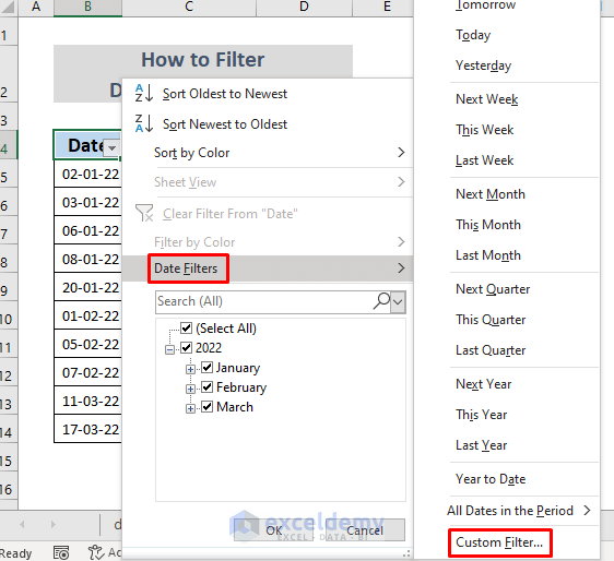
- Set the Date as ‘is before 01-02-22 Or is after 07-02-22’ (see the figure below)
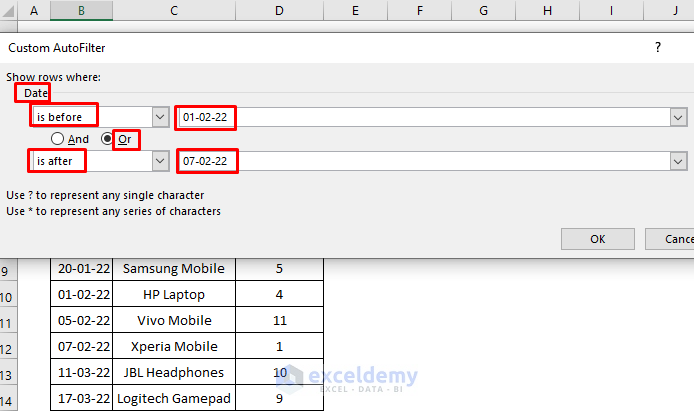
- Click OK and you will see the sales information in the months of January and March.
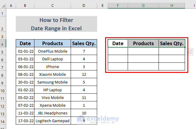
Method 2 – Filtering Dates by Using the FILTER Function
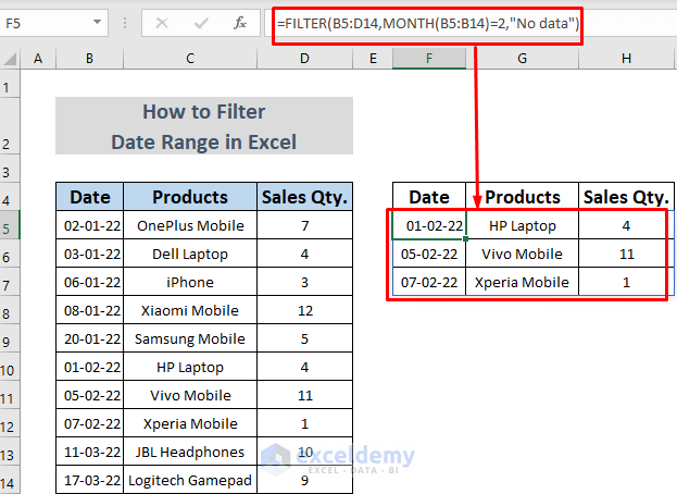
We’ll fetch the sales in February.
Steps:
- Make a new chart like the following figure with the same column headers as the original.
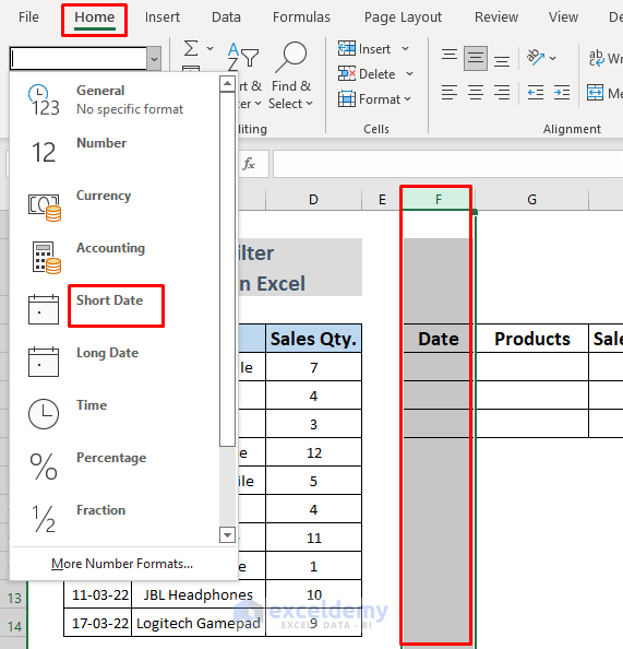
- Make sure that the cell format of column F is set to Date.
- Use the following formula in cell F5.
=FILTER(B5:D14,MONTH(B5:B14)=2,"No data")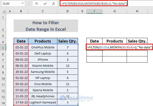
- Press Enter and you will see all the information about product sales in February.
Method 3 – Utilizing a Pivot Table to Filter the Range of Dates
We’ll get the total sales in January.
Steps:
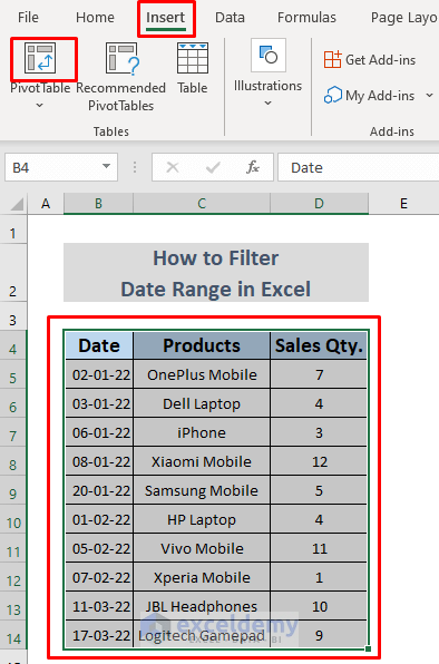
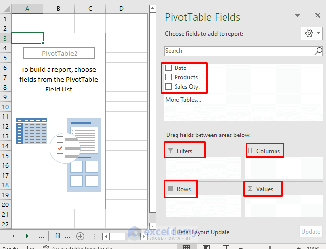
- Select the range B4:D12.
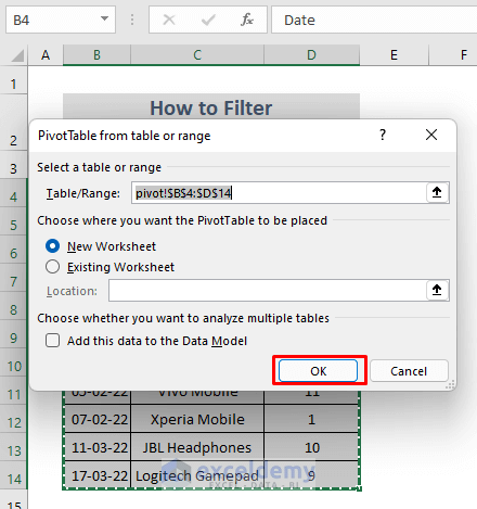
- Go to Insert and select PivotTable.
- A dialog box will pop up. Click OK.
- You will see PivotTable Fields on the right side in a new Excel Sheet. It has all Fields from the Column Headings of your dataset. There are four areas: Filters, Columns, Rows, and Values. You can drag any Field on these Areas.
- Click on Date in the PivotTable Field. You will see another field, Month.
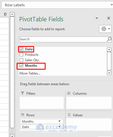
- Unmark Date and mark Products and Sales Qty. from Fields.
- Drag the Months field from the area of Rows to Filters (Shown in the following image).
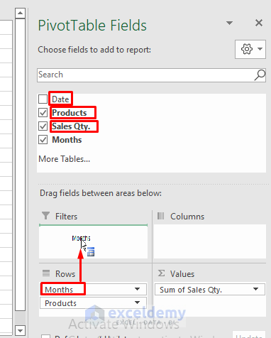
- This will show every Sale and Product of the dataset in a Pivot Table.
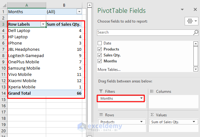
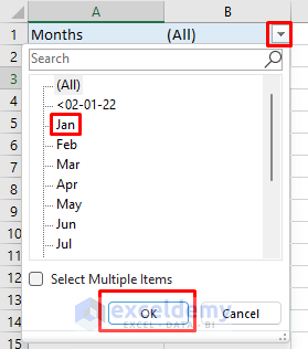
- To see the Sales in January, click on the arrow of the marked area in the following picture, and then select Jan.
- Click OK.
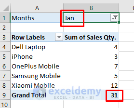
- You can also see the total sales of January.
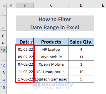
Method 4 – Applying VBA to Filter a Date Range
We’ll get the sales in February and March.
Steps:
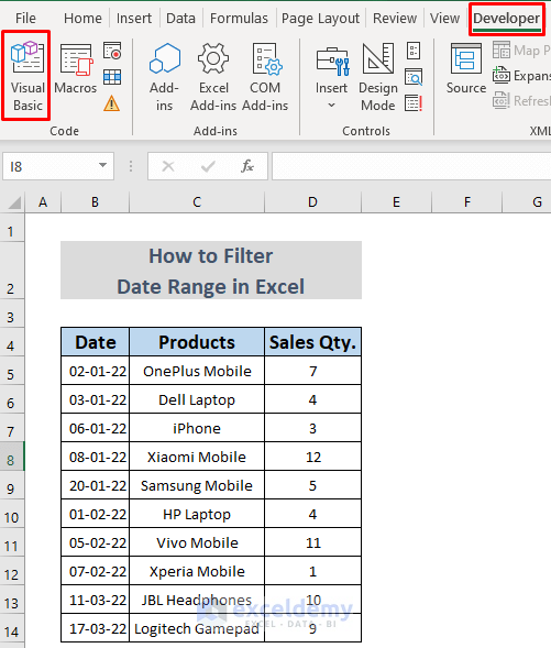
- Open Visual Basic from the Developer Tab.
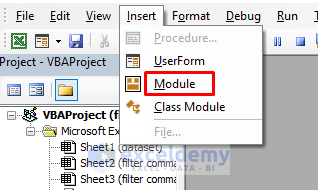
- Open Insert and select Module.
- Use the following code in the VBA Module.
Public Sub DateRangeFilter()
    Dim StartDate As Long, EndDate As Long
    StartDate = Range("B10").Value
    EndDate = Range("B14").Value
    Range("B4:B14").AutoFilter field:=1, _
        Criteria1:=">=" & StartDate, _
        Operator:=xlAnd, _
        Criteria2:="<=" & EndDate
End Sub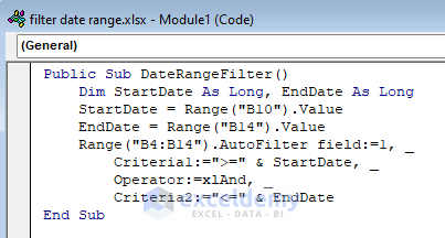
As we want to know about the sales in the months of February and March, we set the first date of February as our start date (cell B10) and the last date of March as our end date (cell B14) using the Range and Value method. Then we used the AutoFilter method to Filter this date range from B4:B14 by setting criteria for the start date and end date.
- Run the Macro from the Excel sheet.
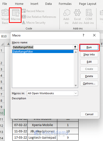
- You will only see the dates of February and March.
Read More: Excel VBA: Filter Date Range Based on Cell Value
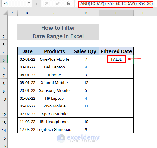
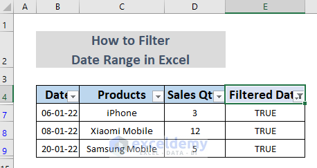
Method 5 – Using Excel AND and TODAY Functions to Filter a Date Range
We want to know the sales history with dates between 60 and 80 days ago from today.
Steps:
- Make a new column and name it as you wish. We named it Filtered Date.
- Use the following formula in cell E5.
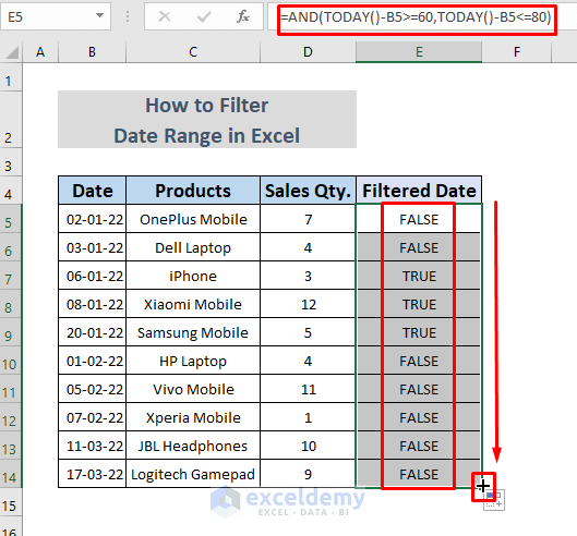
=AND(TODAY()-B5>=60,TODAY()-B5<=80)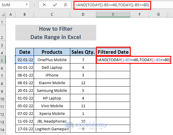
- Hit the Enter key and you will see the output in cell E5.
- Use the Fill Handle to AutoFill lower cells.
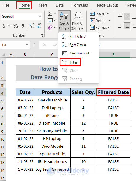
- Select cell E5 and go to Sort & Filter and select Filter.
- Click on the arrow in column E, unmark FALSE, and then click OK (shown in the following figure).
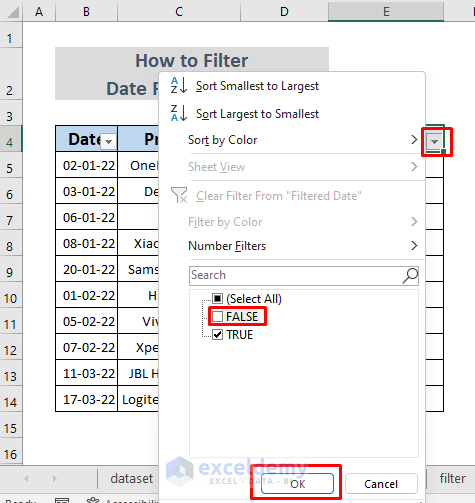
- You will see the sales history among your desired range of dates.
Read More: [Fixed!] Excel Date Filter Is Not Grouping by Month
Practice Section
We’ve provided a practice section in the download file so you can test these methods.
Download the Practice Workbook
Knowledge Hub
<< Go Back to Filter in Excel | Learn Excel
Get FREE Advanced Excel Exercises with Solutions!

That was wonderful! I didn’t expect anybody to be able to help, but your method 5 was perfect for my needs. Thank you!
Thank you Sir! I hope you will find my other articles useful and enjoyable too. Please visit this Link to explore more!