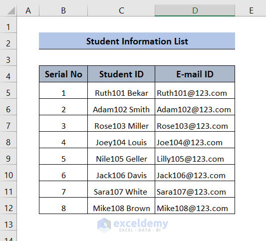
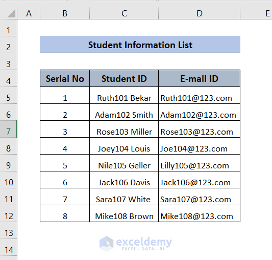
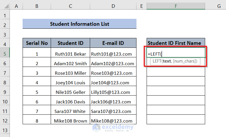
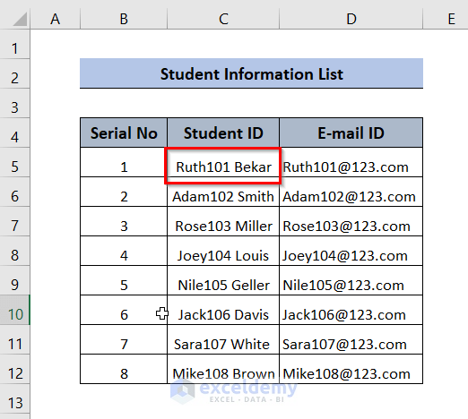
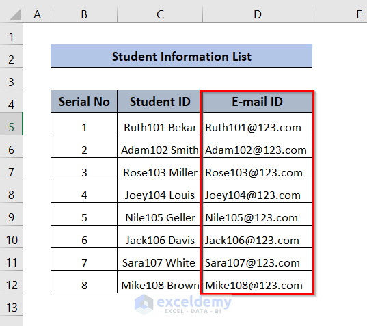
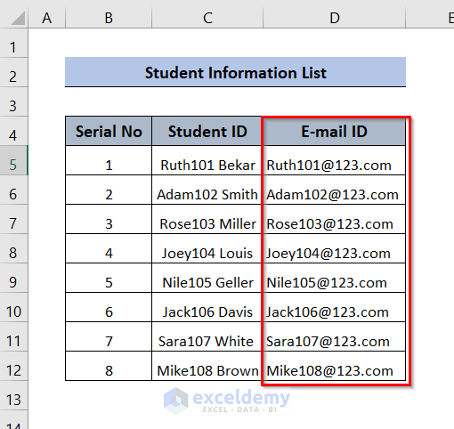
Consider the following Student Information List, which shows Serial No, Student ID, and E-mail ID columns. We will use 5 different methods to extract data from the following table’s cells.
Method 1 – Using the Text to Columns Feature to Extract Data from a Cell
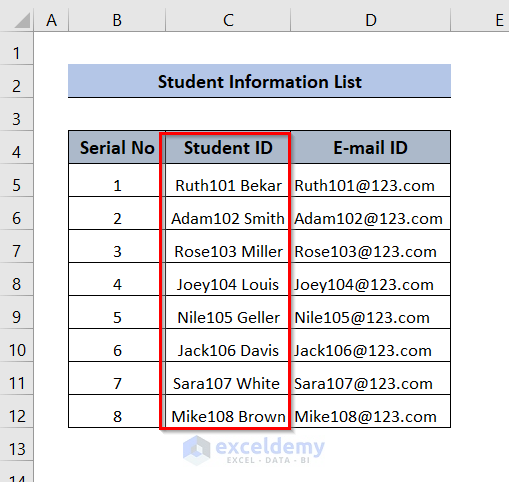
Let’s extract the Student ID in two different cells, splitting the first name and ID from the last name.
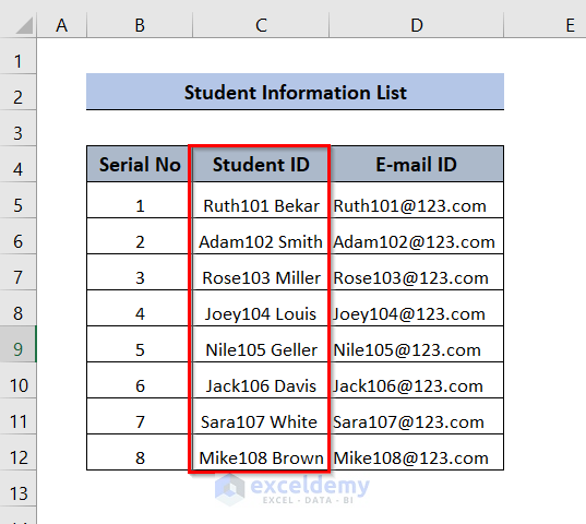
- Select the entire data range of the Student ID column.
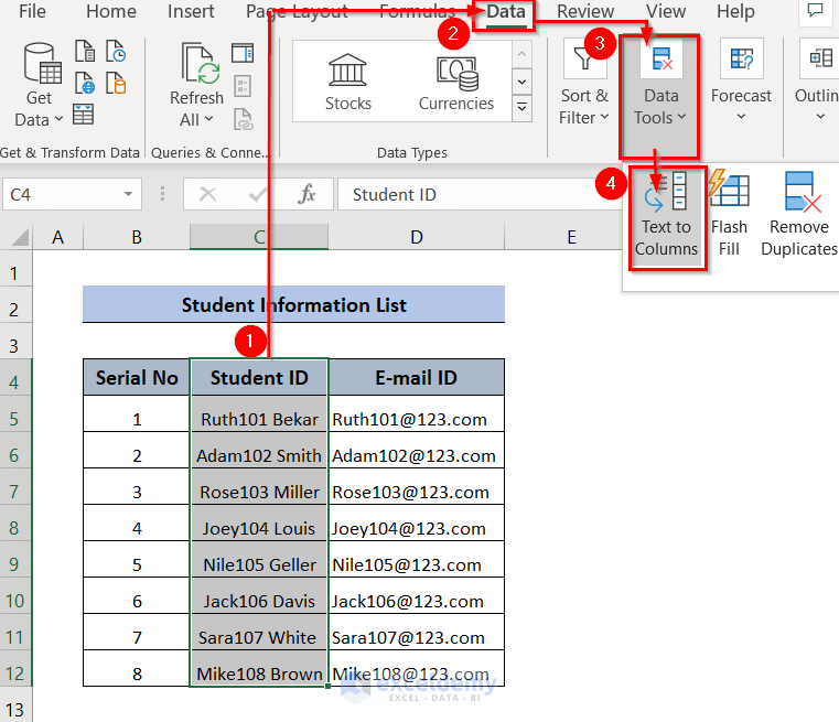
- Go to the Data tab in the Ribbon.
- Click on Data Tools.
- Select the Text to Column option.
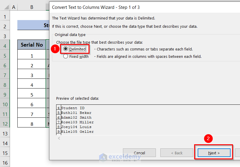
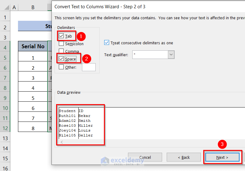
- A Text to Column Wizard window will appear. Select the Delimited option.
- Click on Next.
- Select Tab and Space delimiters. We will see in the Data Preview that there will be a Tab and Space between the data.
- Click Next.
- Provide a destination of the data in the Destination box. We selected cell F4.
- Click Finish.
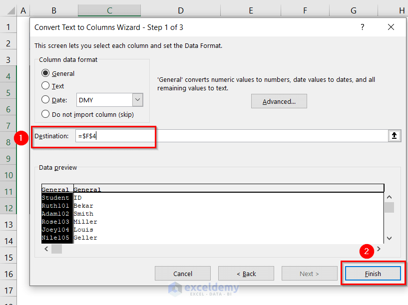
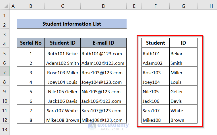
- The Student ID column data is extracted in columns Student and ID.
Read More: How to Extract Data from Excel Sheet
Method 2 – Use Excel Functions to Extract Data from a Cell
In this method, we will use LEFT, RIGHT, and MID functions to extract data from the Student ID column.
LEFT Function
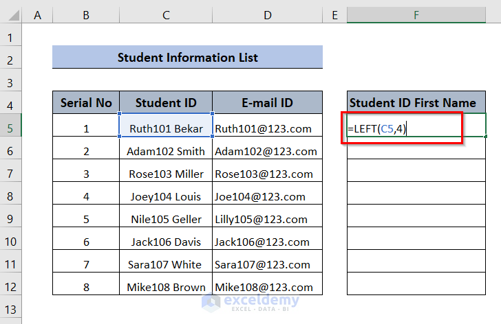
We will extract the first name of the Student ID column using the LEFT function.
- Copy the following formula in cell F5:
=LEFT(C5,4)We have selected the Text in a cell we want to want to extract (in this case, data from cell C5). Then, we have provided the number of characters from the cell, starting from the left, that we want to extract (four since the names have four characters each).
- Press Enter.
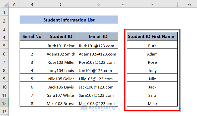
- Drag down the function with the Fill Handle tool.
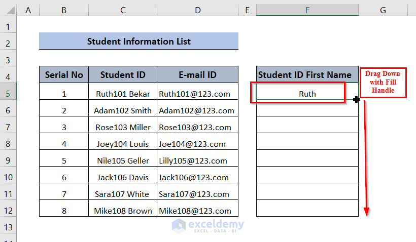
- The column will get filled.
RIGHT Function
We will extract the last name of cell C5 from the Student ID list using the RIGHT function.
- Insert the following formula in F5 (we’re extracting the last five characters since that’s how long the last names are):
=RIGHT(C5,5)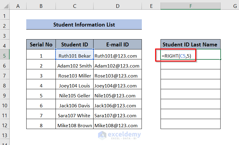
- Press Enter, and you’ll get the last name from cell C5 in the Student ID column in cell F5.
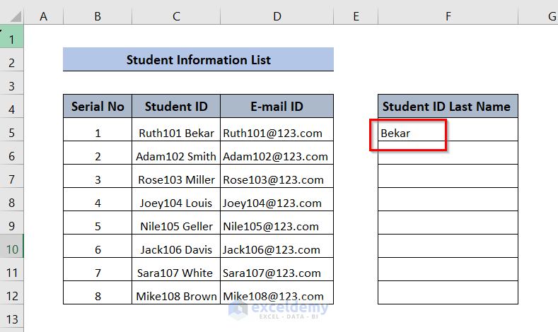
- Use the Fill Handle to fill all the values.
MID Function
Let’s extract the number situated in the middle of the first name and last name of the Student ID column with the MID function.
- Since the number in C5 starts from the fifth position in the string and is three characters long, insert this formula into cell F5:
=MID(C5,5,3)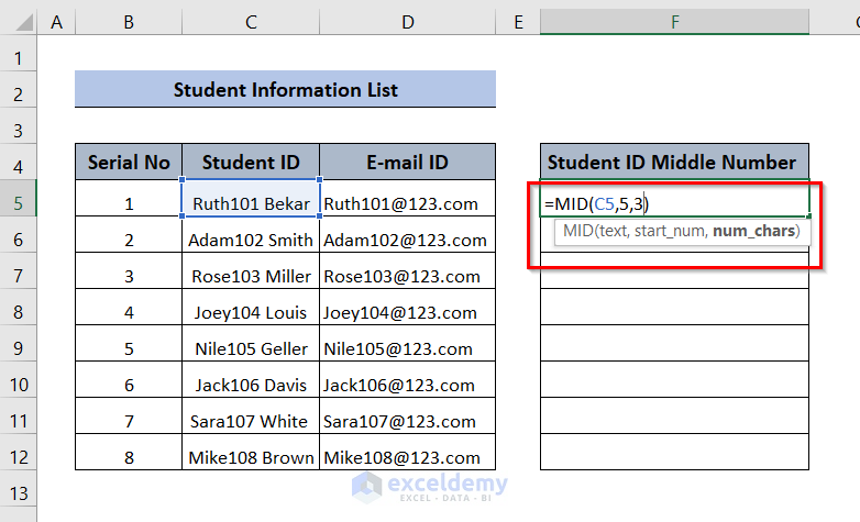
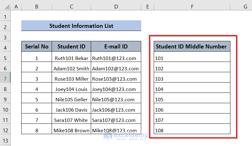
- Press Enter and drag down the function with the Fill Handle tool.
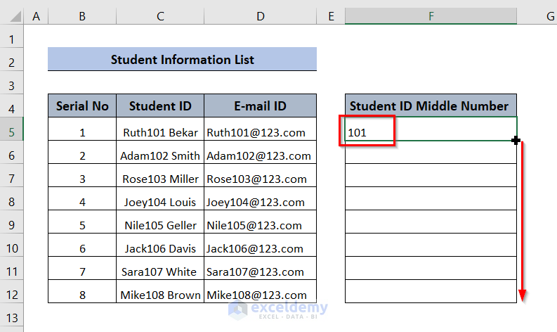
- We can see the results as text strings containing the numbers from Student ID.
Read More: How to Extract Data from a List Using Excel Formula
Method 3 – Combination of LEFT and FIND Functions
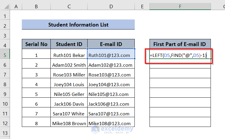
We want to extract the first part with the name and number before “@” from the column E-mail ID.
- Insert the following formula in F5:
=LEFT(D5,FIND("@",D5)-1)- FIND(“@”,D5) → finds the position of @ within D5
Output: 8
- FIND(“@”,D5)-1 → becomes 8-1
Output: 7
- LEFT(D5,FIND(“@”,D5)-1) → turns into LEFT(D5,7)
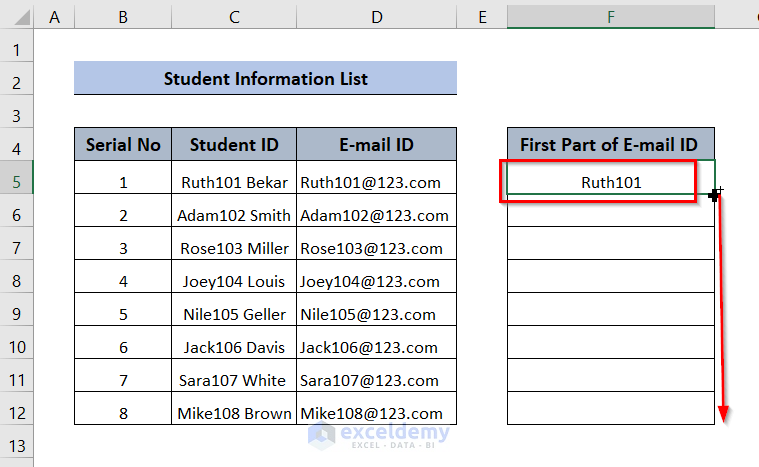
Output: Ruth101
- Press Enter and use the Fill Handle tool to drag down the function.
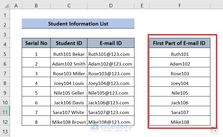
- We can see that the first part of the E-mail ID column has been extracted in the column First Part of E-mail ID.
Read More: How to Extract Data Based on Criteria from Excel
Method 4 – Extract Data Using the VLOOKUP Function
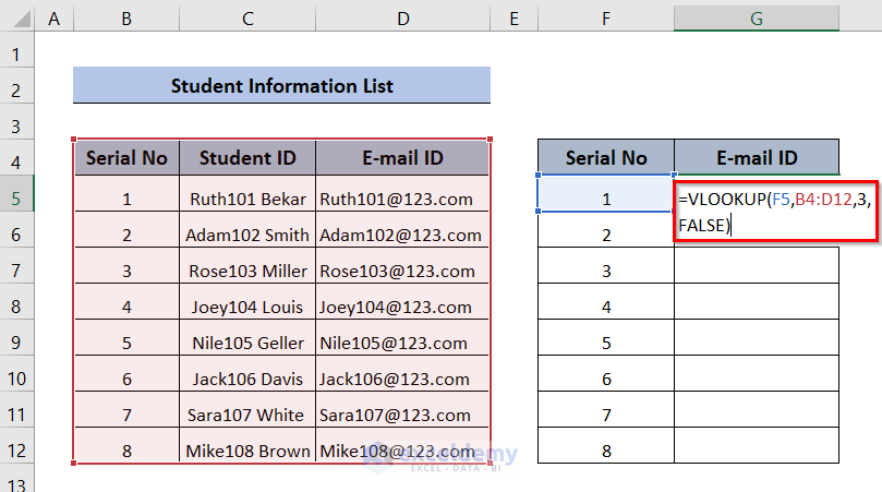
Let’s extract the e-mail ID from E-mail ID column in cell G5 for Serial No 1 using the VLOOKUP function.
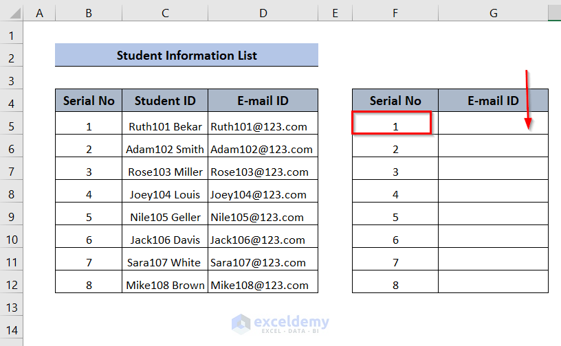
- Insert the following formula in Cell G5.
=VLOOKUP(F5,$B$4:$D$12,3,FALSE)We put F5 as the lookup value, selected B4:D12 as the table array, used column Index as 3, and chose False for an exact match.
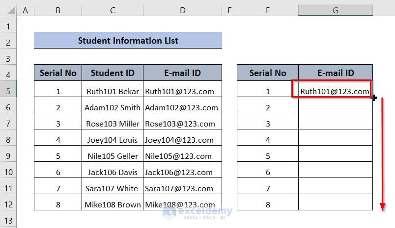
- Press Enter to get the result.
- Drag down the function with the Fill Handle tool.
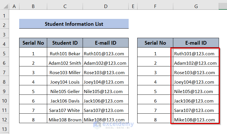
- We can see extracted e-mail id in column E-mail ID. You can change the numbers in column F and get the corresponding results.
Read More: How to Extract Specific Data from a Cell in Excel
Method 5 – INDEX-MATCH to Extract Data from a Cell
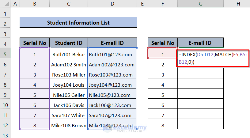
Let’s extract the e-mail id from E-mail ID column in cell G5 for Serial No 1 using the INDEX & MATCH functions.
- Insert the following formula in cell G5:
=INDEX($D$5:$D$12,MATCH(F5,$B$5:$B$12,0))For the INDEX function, we provided the array from D5 to D12. The value to search is provided by the MATCH function’s result.
In the MATCH function, we give lookup_value as F5. The lookup_array is from B5 to B12. The match_type is 0 for exact matches.
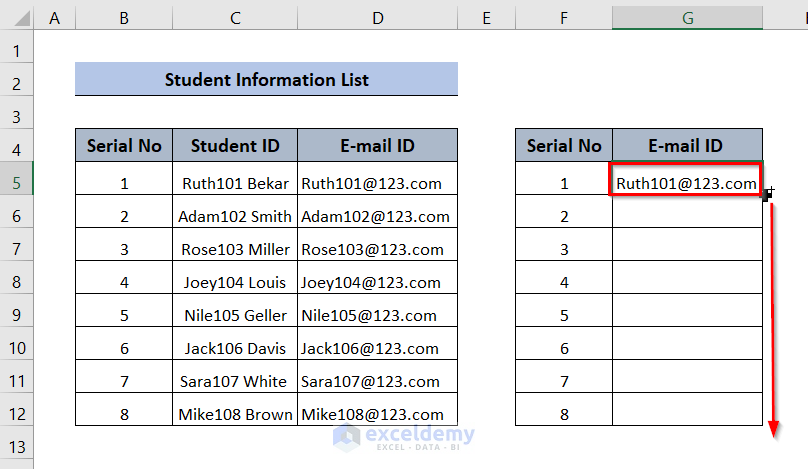
- Press Enter to get the first result.
- Drag down the function with the Fill Handle tool.
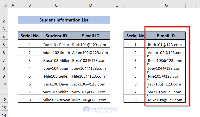
- We can see the extracted e-mail IDs in column E-mail ID.
Download Workbook
Related Articles
- Excel Formula to Get First 3 Characters from a Cell
- How to Extract Month and Day from Date in Excel
- How to Extract Month from Date in Excel
- How to Extract Year from Date in Excel
- How to Extract Data From Table Based on Multiple Criteria in Excel
<< Go Back To Extract Data Excel | Learn Excel
Get FREE Advanced Excel Exercises with Solutions!
