Extract Filtered Data in Excel to Another Sheet: 4 Methods

Method 1 – Extract Filtered Data to Another Sheet Using Copy-Paste Method in Excel

If you don’t need to perform additional table transformations after extracting data in Excel to another sheet, you can use the Copy-Paste method for that. Follow these steps.

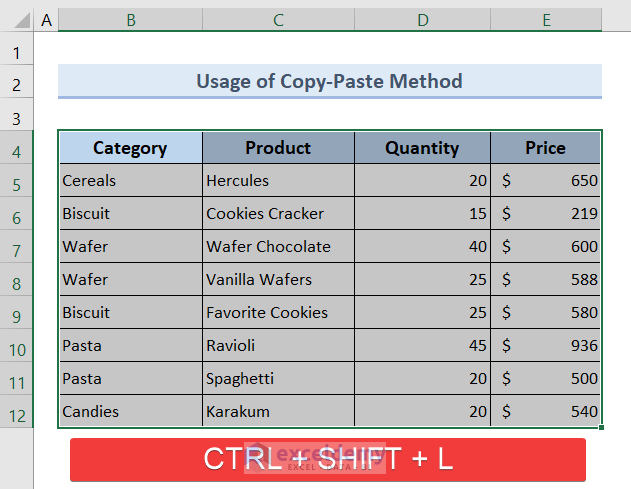
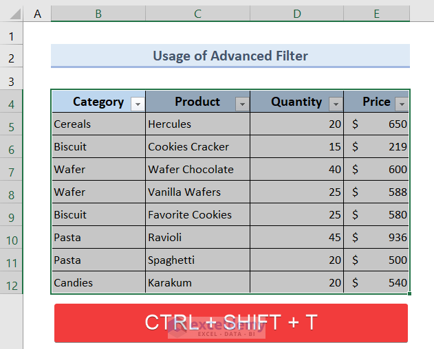
❶ Select the whole dataset and press CTRL + SHIFT + L to apply Filter.

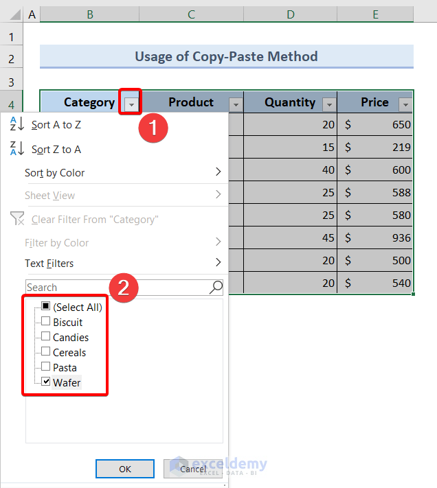
❷ Click on a drop-down icon at the bottom-right corner of the column headers.

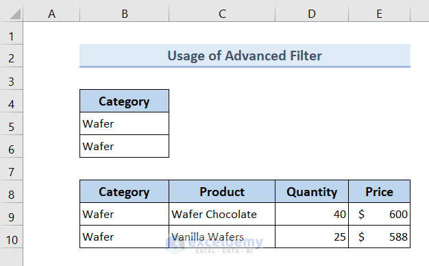
❸ Pick an item from the list. Let’s go with Wafer for now.

❹ Hit the OK button.

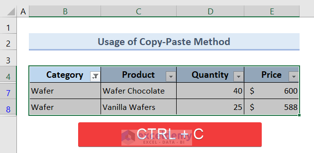
This will present only the filtered data based on the criteria and other rows will be hidden.

❺ Press CTRL + C to Copy them all into the clipboard.

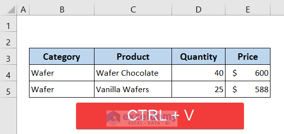
❻ Open a different worksheet in Excel, then press CTRL + V to Paste the selection.

Read More: How to Get Data from Another Sheet Based on Cell Value in Excel

Method 2 – Extract Filtered Data to Another Sheet in Excel Using Advanced Filter

The Advanced Filter allows you to use a smaller table to filter by and fill it in. Here’s how:

❶ Select the whole dataset and press CTRL + SHIFT + L to apply Filter.

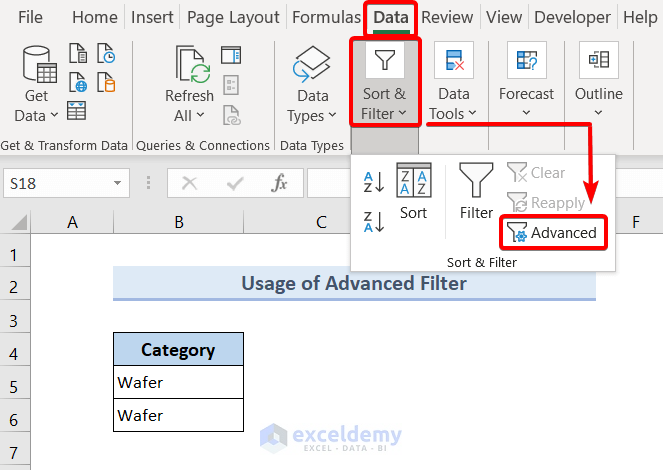
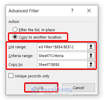
❷ Go to the destination worksheet and input your criteria columns or rows. Now go to Data >> Sort & Filter >> Advanced.

The Advanced Filter dialog box will appear.

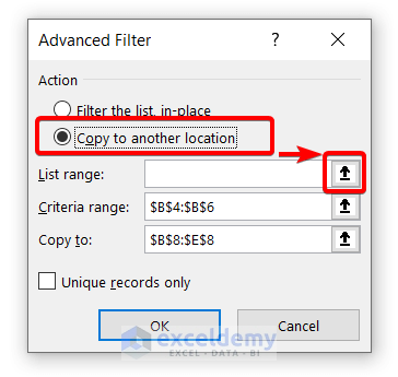
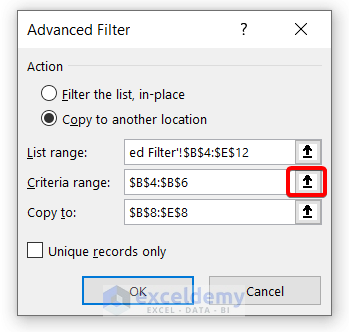
❸ Choose Copy to another location under the Action section. Click on the up arrow icon next to the List range bar.

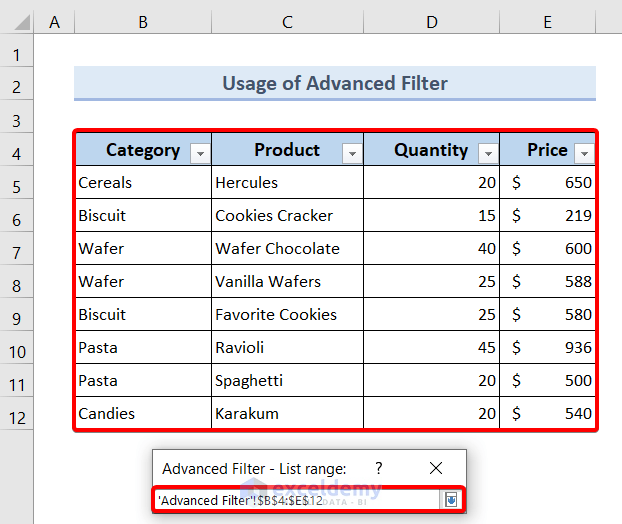
❹ Go back to the worksheet with the original dataset and select the entire dataset. Then, click on the down arrow icon from the Advanced Filter – List range dialog box to go back to the Advanced Filter menu.

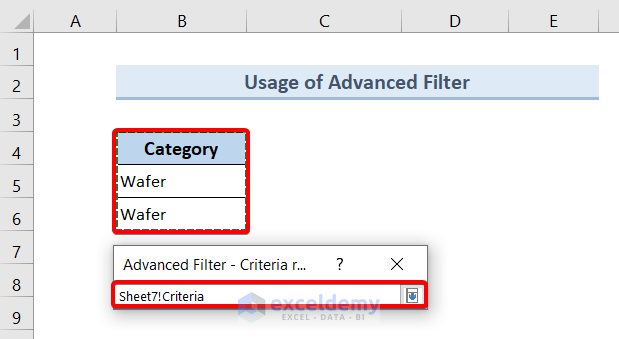
❺ Click on the up arrow icon next to the Criteria range bar.

❻ Select the cell range with the criteria and click on the down arrow icon from the Advanced Filter – Criteria range dialog box.

❼ Finally click on the up arrow icon at the end of the Copy to bar.

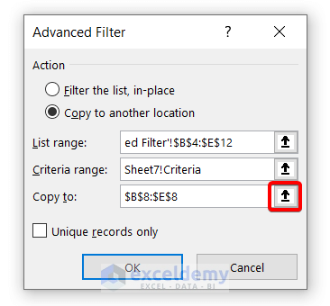
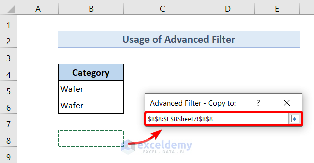
❽ Select a cell on the destination worksheet to store the filtered data then click on the down arrow icon from the Advanced Filter – Copy to: dialog box.

❾ Make sure everything is filled in the Advanced Filter dialog box and hit the OK button.

After that, the filtered data will be extracted to the destination worksheet.

Read More: How to Pull Data from Multiple Worksheets in Excel

Method 3 – Dynamically Extract Filtered Data to Another Sheet in Excel Using Power Query

If you want to extract the filtered data to another sheet and create a dynamic link between them then you can use Power Query.

To do that follow the steps below.

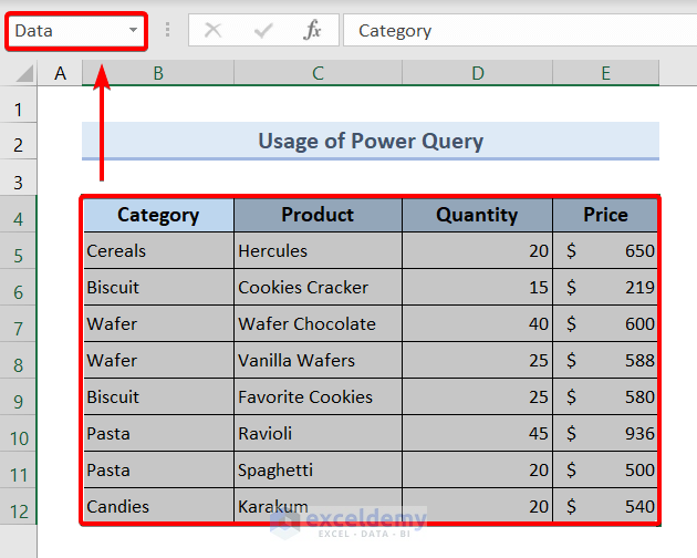
❶ Start by selecting the whole dataset and go to the name box to give the array a name such as Data.

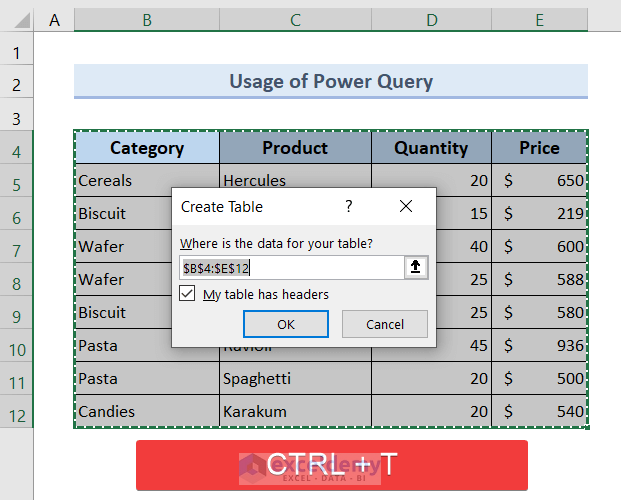
❷ Select the whole data table again and press CTRL + T to convert the dataset into an Excel table. The Create Table dialog box will appear. Just click OK on it.

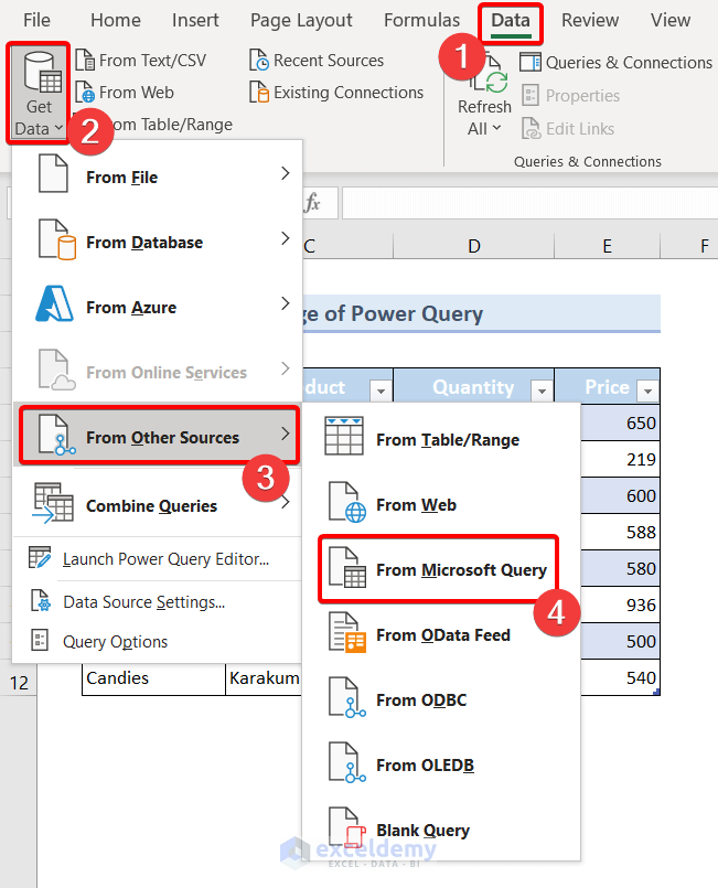
❸ Now go to Data >> Get Data >> From Other Sources >> From Microsoft Query.

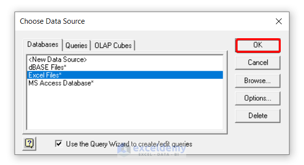
Choose Data Source dialog box will appear.

❹ Select Excel Files and hit OK.

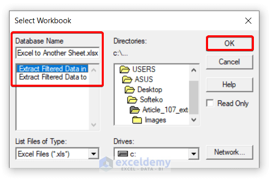
The Select Workbook dialog box will appear.

❺ Select your Excel worksheet name under the Database Name section and hit OK.

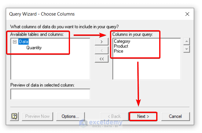
The Query Wizard –  Choose Columns dialog box will appear.

Click on the name and data that you have created previously. This will show all the column names of your dataset.

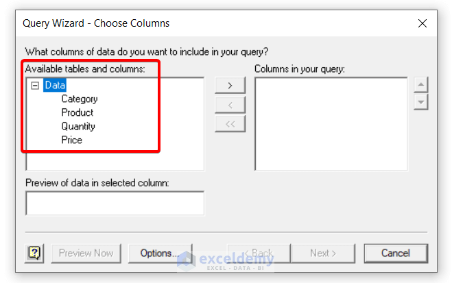
❻ Double click on the column names under the Data in the Available tables and columns section. Those column names will appear in the Columns in your query box. After that hit the Next button to proceed.

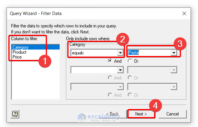
❼ Select a column name from the Column to filter box. Then choose equals from the Only include rows where drop-down. Then from the next drop-down choose an entity to use for comparison, such as Pasta for Category.

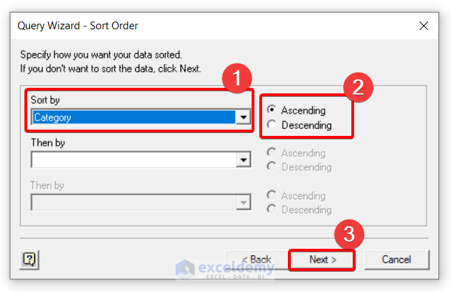
❽ In the next dialog box called Query Wizard – Sort Order, select a column name from the Sort by drop-down. Then choose either Ascending or Descending. After that, you can click on the Next button.

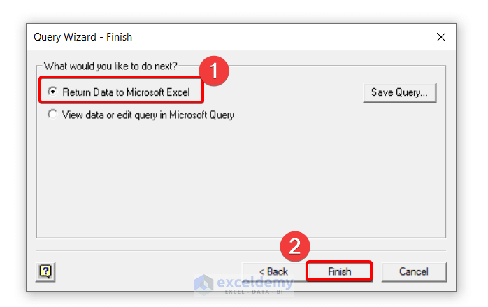
❾ Choose Return Data to Microsoft Excel option from the Query Wizard – Finish dialog box and hit the Finish button.

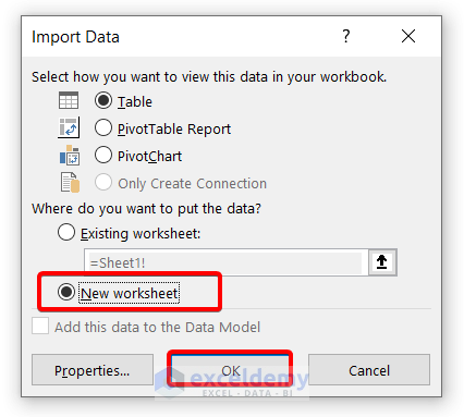
After that, the Import Data dialog box will appear.

❿ Choose the New worksheet option and hit OK.

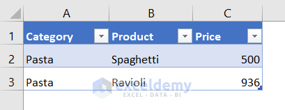
Finally, you will get the filtered data extracted in a new worksheet like this.

Read More: How to Pull Values from Another Worksheet in Excel

Method 4 – Use VBA Script to Extract Filtered Data to Another Sheet in Excel

To use a VBA code to extract filtered data to another sheet in Excel, go through the following steps.

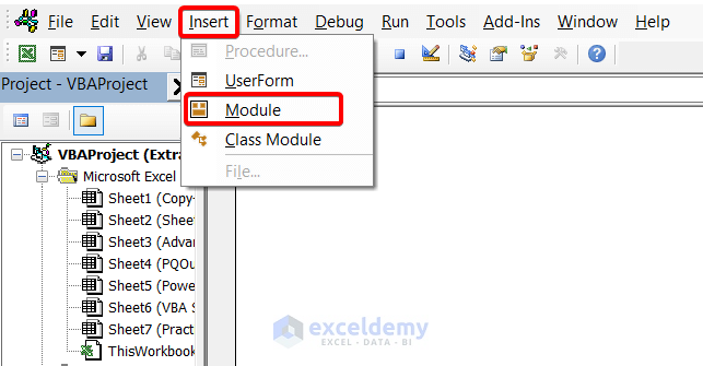
❶ Press ALT + F11 to open the VBA editor.

❷ Go to Insert > Module.

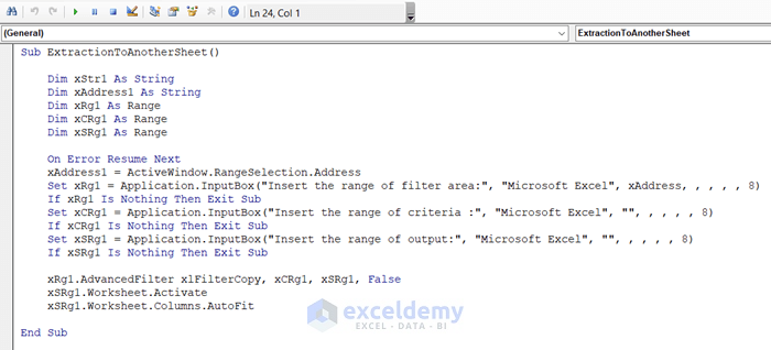
❸ Copy and paste the following VBA code:

Sub ExtractionToAnotherSheet()

    Dim xStr1 As String
    Dim xAddress1 As String
    Dim xRg1 As Range
    Dim xCRg1 As Range
    Dim xSRg1 As Range

    On Error Resume Next
    xAddress1 = ActiveWindow.RangeSelection.Address
    Set xRg1 = Application.InputBox("Insert the range of filter area:", "Microsoft Excel", xAddress, , , , , 8)
    If xRg1 Is Nothing Then Exit Sub
    Set xCRg1 = Application.InputBox("Insert the range of criteria :", "Microsoft Excel", "", , , , , 8)
    If xCRg1 Is Nothing Then Exit Sub
    Set xSRg1 = Application.InputBox("Insert the range of output:", "Microsoft Excel", "", , , , , 8)
    If xSRg1 Is Nothing Then Exit Sub

    xRg1.AdvancedFilter xlFilterCopy, xCRg1, xSRg1, False
    xSRg1.Worksheet.Activate
    xSRg1.Worksheet.Columns.AutoFit

End Sub

❹ Paste and Save the VBA code in the VBA editor.

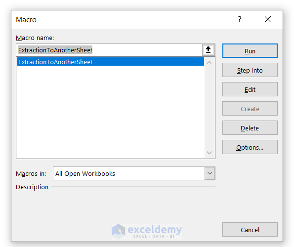
❺ Go back to the worksheet and press ALT + F8 to call up the Macro dialog box. Then hit the Run button.

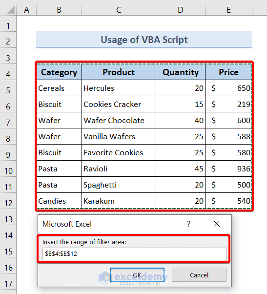
A small Input Box will appear.

❻ Insert the range of the filter area into that input box.

❼ Here, I selected the range B4:E12. Then click OK.

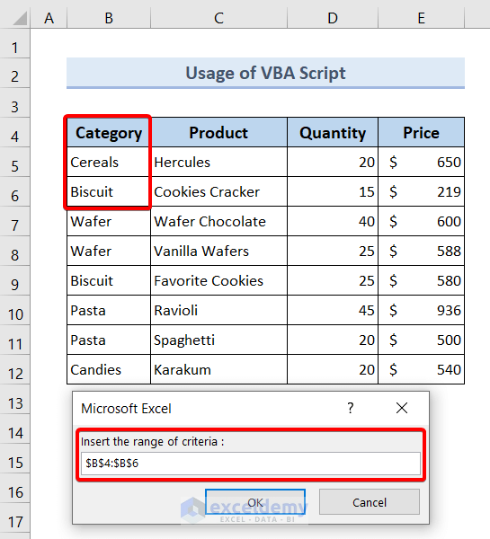
Another Input Box will appear.

❽ Insert the cell range of the criteria into that input box and hit OK.

❾ Then in the last Input Box, insert the destination cell ranges from a different worksheet. Then click OK.

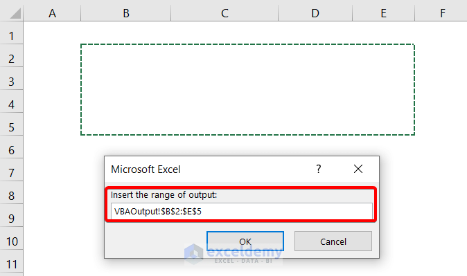
After that, you will get the filtered data in your preferred cell range in the second worksheet.

Read More: How to Pull Data From Another Sheet Based on Criteria in Excel

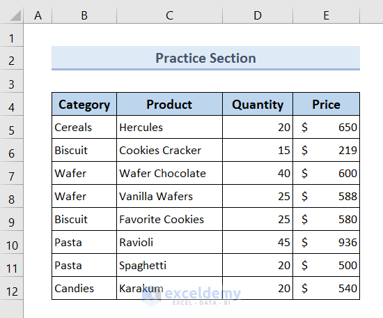
Practice Section

Here’s a basic worksheet that details foodstuff categories in store and their prices, which you can download below. The instructional steps above used the “Category” as the filter, so try to use a different column such as quantity or price to create new tables using the more advanced methods.

Download Practice Workbook

You can download the Excel file from the following link and practice along with it.

Related Articles

• Pull Same Cell from Multiple Sheets into Master Column in Excel
• How to Pull Data from Multiple Worksheets in Excel VBA
• Excel Macro: Extract Data from Multiple Excel Files
• How to Pull Data from Multiple Worksheets in Excel

<< Go Back To Extract Data Excel | Learn Excel