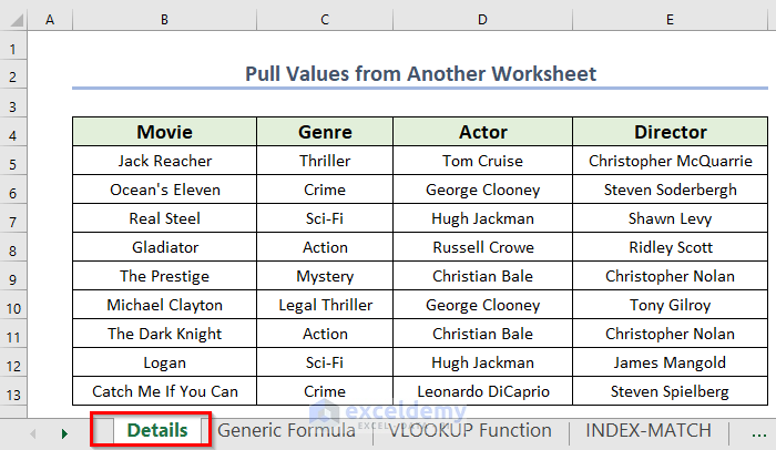
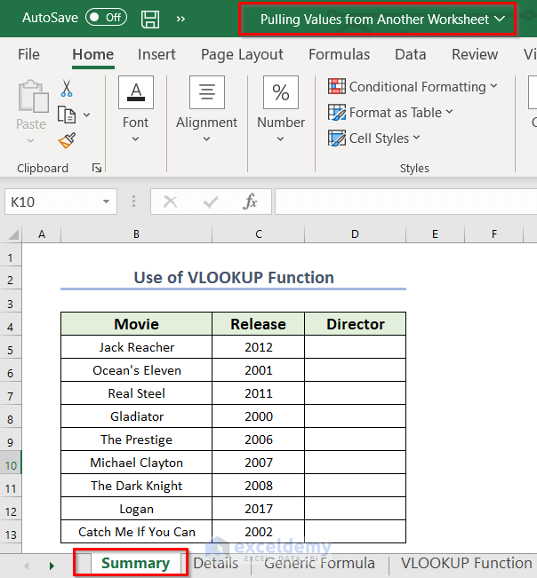
We have a table with movie information in the sheet called Details. We will pull values from this table to the other worksheets.
Method 1 – Use a Generic Formula with Cell References to Insert Values
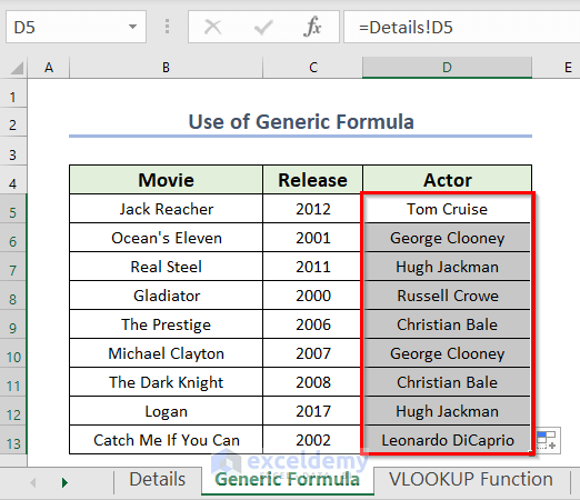
You can pull values from another worksheet by providing the cell reference that contains the sheet name in the formula.
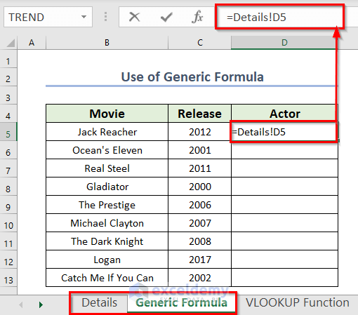
We have put a column Actor in the worksheet named Generic Formula. We want to pull the actor names for the respective movies from the worksheet named Details.
- In cell D5, use the following formula:
=Details!D5Details is the sheet name and D5 is the cell reference. Insert an exclamation “!” sign between the sheet name and cell reference.
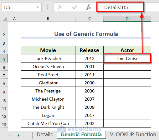
- Press Enter.
- Double-click on the Fill Handle icon.
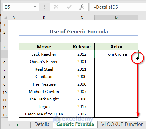
- We get the names of all actors. Since the data is in the same sequence in both of the sheets, we get the names in the correct order.
Read More: How to Pull Data From Another Sheet Based on Criteria in Excel
Method 2 – Use the VLOOKUP Function to Pull Values from Another Worksheet
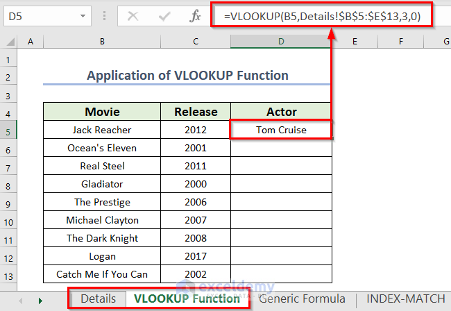
- Use the following formula in cell D5 in the sheet named VLOOKUP Function:
=VLOOKUP(B5,Details!$B$5:$E$13,3,0)- Press Enter to get the result. This pulled the actor of the movie Jack Reacher from the Details sheet.
Formula Breakdown
- We have provided B5 as the lookup_value within the VLOOKUP function, and Details!$B$5:$E$13 is the lookup_array. You can notice we have provided the sheet name before the range. Moreover, the sheet name and range are separated by the “!” sign.
- 3 is the col_index_num because actors are in the 3rd column of the range.
- 0 for the exact match.
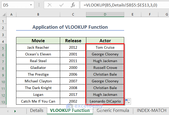
- Double-click on the Fill Handle icon to AutoFill the corresponding data in the rest of the cells D6:D13.
Read More: How to Pull Data from Multiple Worksheets in Excel VBA
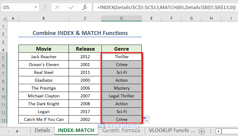
Method 3 – Combine Excel INDEX and MATCH Functions to Place Values
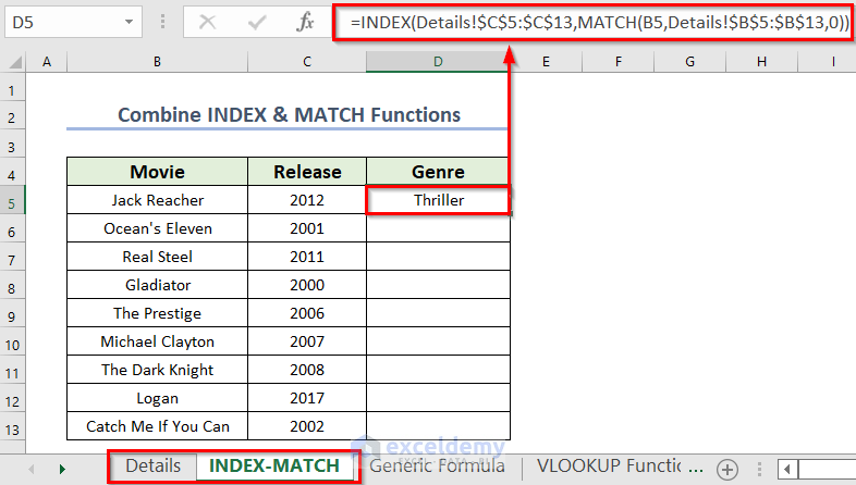
We’ll get the genres of the movies.
- Use the following formula in the D5 cell of the INDEX-MATCH sheet.
=INDEX(Details!$C$5:$C$13,MATCH(B5,Details!$B$5:$B$13,0))- Press Enter.
Formula Breakdown
- Within the MATCH function, B5 is the lookup_value, and Details!$B$5:$B$13 is the lookup_range.
- This MATCH portion provides the position.
- INDEX pulls the value from the Details!$C$5:$C$13 range.
- Use the AutoFill feature for the rest of the values.
Read More: Extract Filtered Data in Excel to Another Sheet
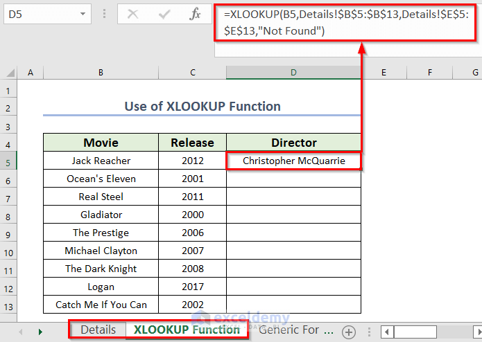
Method 4 – Apply Excel XLOOKUP Functions to Insert Values from Another Worksheet
If you are using Excel 365, you can use XLOOKUP to pull the values, which is an improved version of VLOOKUP since it can fetch values to the left of the lookup range.
- Use the following formula in the D5 cell of the XLOOKUP Function sheet:
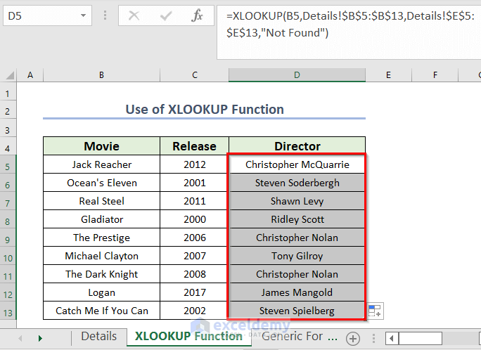
=XLOOKUP(B5,Details!$B$5:$B$13,Details!$E$5:$E$13,"Not Found")- Hit Enter.
Formula Breakdown
- B5 is the lookup_value, Details!$B$5:$B$13 is the lookup_range, and Details!$E$5:$E$13 is the range from which we need to pull values. We have written the sheet reference, Details!, for each of the ranges.
- We have added “Not Found” to the optional field if_not_found.
- Repeat for other cells or use AutoFill.
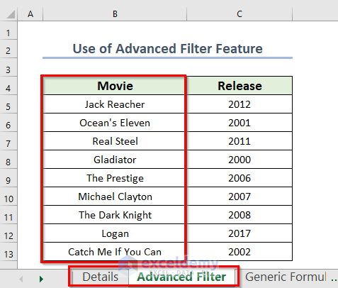
Method 5 – Use the Advanced Filter for Pulling Values from Another Worksheet
We want to pull all the values from the worksheet Details for the movie names.
- Write down the criteria, including that particular column header. We have written the names of the movies in the B5:B13 cells under the Movie column.
- Open the Advanced Filter option by clicking the Data tab and going to Sort & Filter then choosing Advanced.
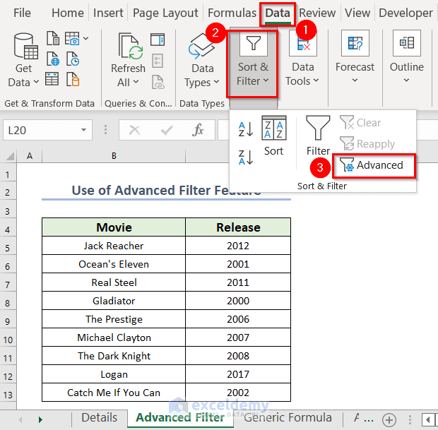
- You will see a new dialog box named Advanced Filter.
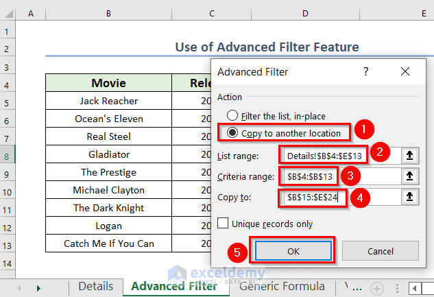
- Mark Copy to another location.
- Specify the range (Details!$B$4:$E$13) in the List range option from where you want to pull the values (worksheet named Details).
- Provide the criteria ($B$4:$B$13) in the Criteria range box.
- Choose the space ($B$15:$E$24) in the Copy to box. You must select a space up to which you need.
- Press OK.
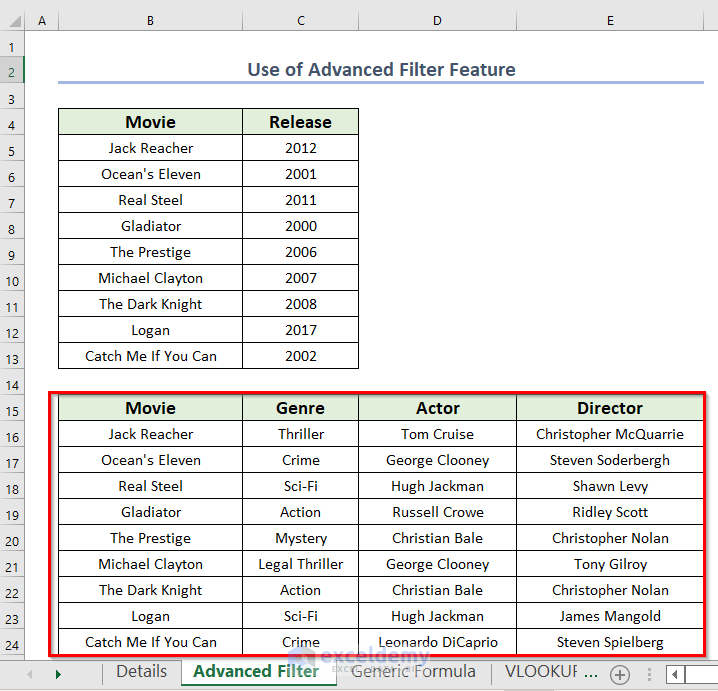
- You’ll get the following output.
Method 6 – Use the VLOOKUP Function to Pull Values from a Different Workbook in Excel
We have copied the Details sheet value to another workbook called Use Another Workbook.xlsx. We have set the name of the sheet as Details in New Workbook.
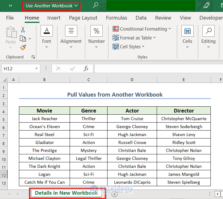
Our summary table (worksheet name Summary) is still in the workbook Pulling Values from Another Worksheet.xlsx. We will pull the director’s name from the workbook named Use Another Workbook.
You can use any of the approaches (Cell Reference, VLOOKUP, INDEX-MATCH, XLOOKUP) mentioned above by changing the reference to select a different workbook.
- Use the following formula.
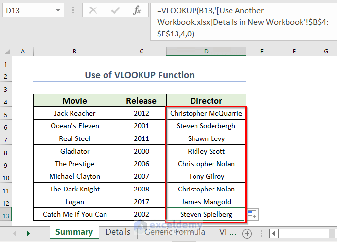
=VLOOKUP(B5,'[Use Another Workbook.xlsx]Details in New Workbook'!$B$4:$E$13,4,0)- Press Enter.
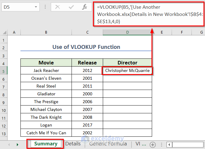
Formula Breakdown
- For the the cell range $B$4:$E$13 we have provided the sheet name (Details in New Workbook) and the workbook name (Use Another Workbook.xlsx). The workbook name is in the brackets.
- We need to count the workbook and worksheet simultaneously, so they are within single quotes (‘).
- Repeat for the rest of the values or use the AutoFill feature.
Read More: Pull Same Cell from Multiple Sheets into Master Column in Excel
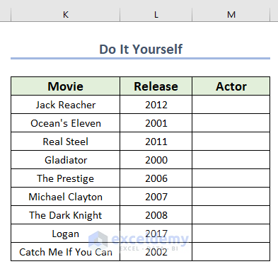
Practice Section
You can practice the explained methods by yourself in the download file.
Download the Practice Workbook
Related Articles
- Extract Data from One Sheet to Another Using VBA in Excel
- How to Get Data from Another Sheet Based on Cell Value in Excel
- Excel Macro: Extract Data from Multiple Excel Files
- How to Pull Data from Multiple Worksheets in Excel
<< Go Back To Extract Data Excel | Learn Excel
Get FREE Advanced Excel Exercises with Solutions!
