How to Extract Data from a List Using Excel Formula (5 Methods)

Method 1 – Combine INDEX, MATCH, and COUNTIF Functions to Extract Unique Values from a List

We have a dataset containing some names. We will extract unique names from the list.

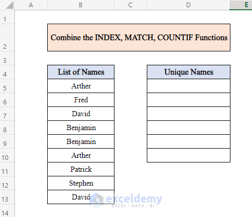
Steps:

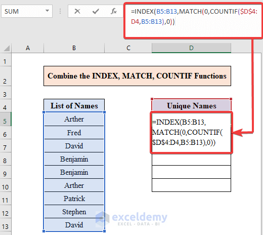
• Click on the first cell (D5) where you want the result.
• Apply the following formula:

INDEX(B5:B13)= Retrieves values to add to the unique list.

COUNTIF($D$4:D4,B5:B13)= Counts unique values contained in the range.

The MATCH Function finds the exact match & zero values for the function.

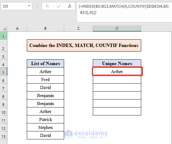
• Press Ctrl + Shift + Enter to apply it. You’ll get the first result.

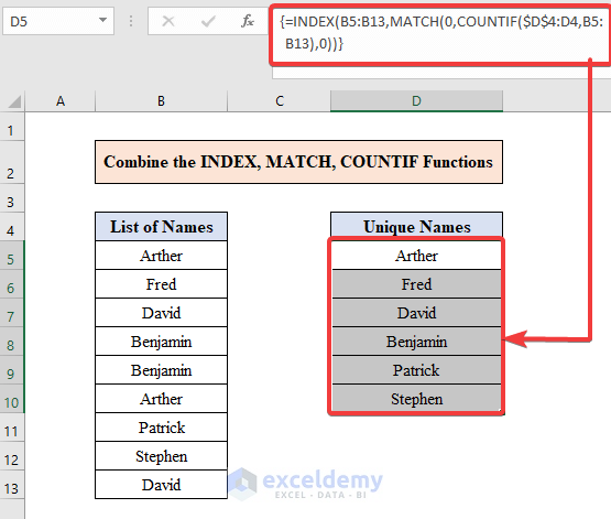
• Drag down the cell using AutoFill.

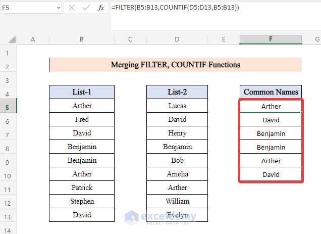
Method 2 – Merge FILTER and COUNTIF Functions to Extract Common Values from a List in Excel

We will find common names in different columns from the two lists.

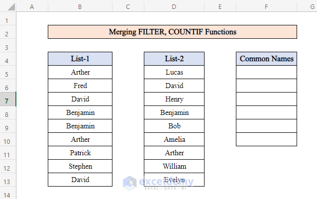
Steps:

• Select cell F5.
• Apply this formula:

COUNTIF(D5:D13,B5:B13)= Takes List-2 (D5:D13) as range and List-1 (B5:B13) as criteria and counts common items. The Filter Function filters value got from the COUNTIF Function.

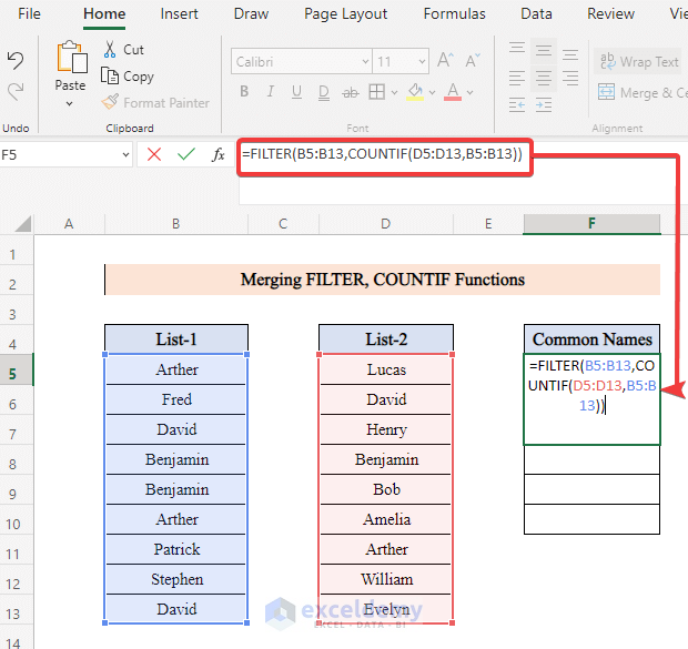
• Pressing Enter gets only one name in the desired column.
• Drag down the Fill Handle to find all the common names from both lists.

Method 3 – Apply an Array Formula to Extract Data from a List Based on Criteria

Case 3.1 – Extract Data from a List Based on Single Criteria

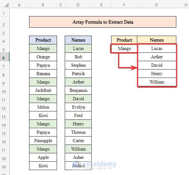
We have a dataset containing one list with Products and another list with product owner Names. In the other two columns, results will be shown. We will find the names that correspond to the product named Mango.

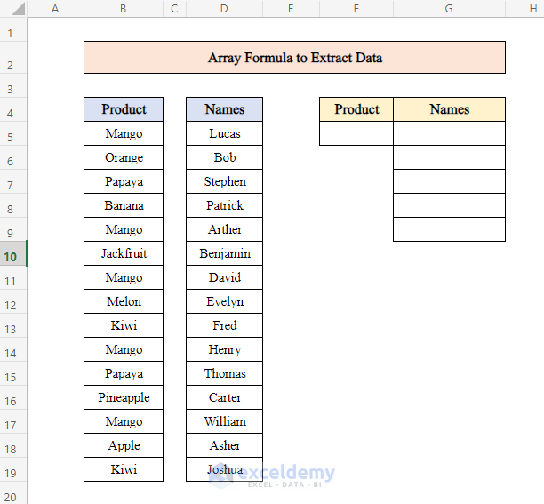
Steps:

• Select cell G5.
• Enter the following formula:

IF($F$5=$B$5:$B$19, COUNTIF($G$4:$G4, $D$5:$D$19) works as the lookup array. The COUNTIF($G$4:$G4, $D$5:$D$19) part filters the data where $G$4:$G4 is the range and $D$5:$D$19 is the criteria. We want the exact match, so we select 0. The INDEX function introduces a range for the IFERROR Function and the MATCH function returns the position of the item in the range.

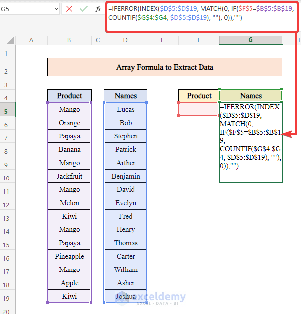
• Press Ctrl + Shift + Enter to see the results.
• In the Output product column, we can put any product from our list. It will show the names related to the product. We have put “Mango” in the output product column.

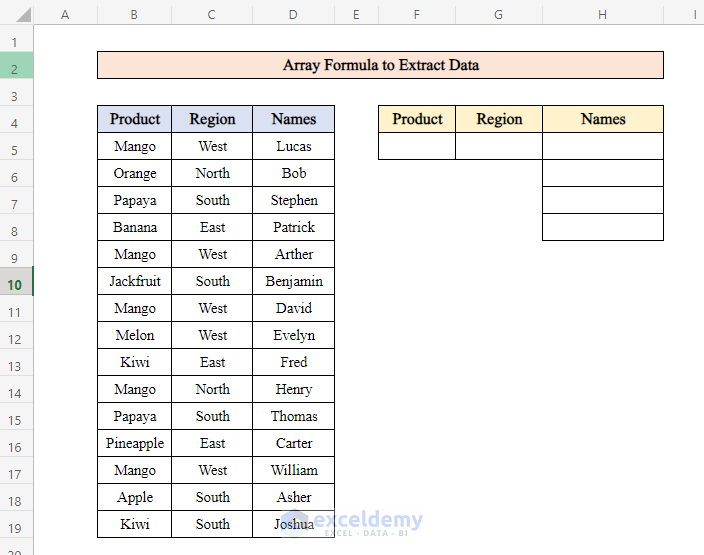
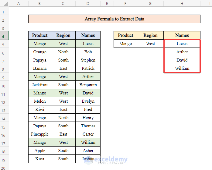
Case 3.2 – Extract Data from a List Based on Multiple Criteria

We have taken three columns containing Product, Region, and Names. On the right side, we’ll use both product and region as criteria.

Steps:

• Select cell H5 where the output will be shown.
• Enter the following formula:

IF($B$5:$B$19<>$F$5,1,0)+IF($C$5:$C$19<>$G$5,1,0),0)= working as a lookup array.

COUNTIF(H4:$H$4,$D$5:$D$19)= This part filters the data where (H4:$H$4) works as range and ($D$5:$D$19) works as criteria. For the exact match, we use 0.

The INDEX function introduces a range for the IFERROR Function and the MATCH function returns the position of the item in the range.

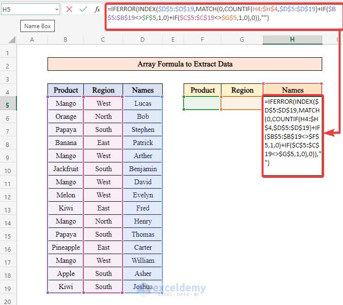
• Pressing Ctrl + Shift + Enter applies the formula and returns all the results.
• If we choose a product and a region, this formula will filter the list and show the names related to these multiple criteria.

Read More: How to Extract Data From Table Based on Multiple Criteria in Excel

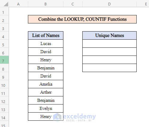
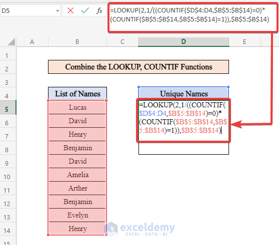
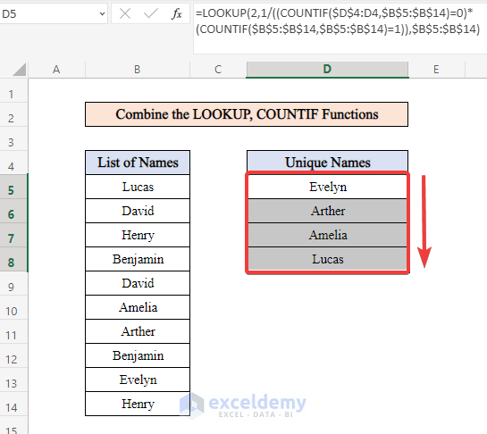
Method 4 – Combine the LOOKUP and COUNTIF Functions to Extract Data from a List in Excel

In the following dataset, we duplicated some names, so we’ll extract the unique values.

Steps:

• Select cell D5.
• Enter the following formula in the cell:

The COUNTIF Function counts each value and returns values. The LOOKUP Function will match the value in the array and return in the result range.

• Press Enter to get the first name in the list.

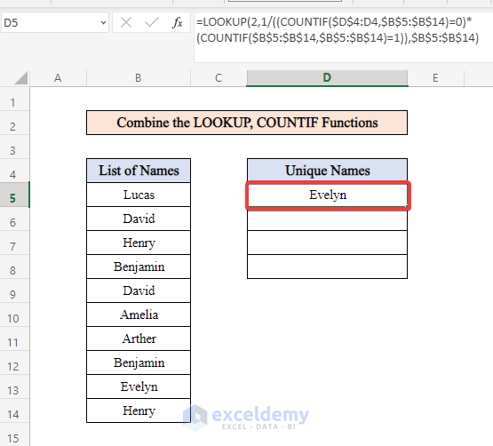
• Drag down using the AutoFill feature until you start getting error values.

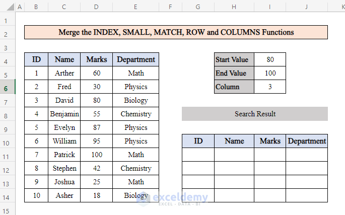
Method 5 – Merge INDEX, SMALL, MATCH, ROW, and COLUMNS Functions to Extract Data from a List

The following dataset contains student information. We took a range of marks from 80 to 100. Students whose marks are between 80 to 100 will be shown in the output column.

Steps:

• The starting value is 80 and the end value is 100.
• As marks are in the third column, we put 3 in the I6

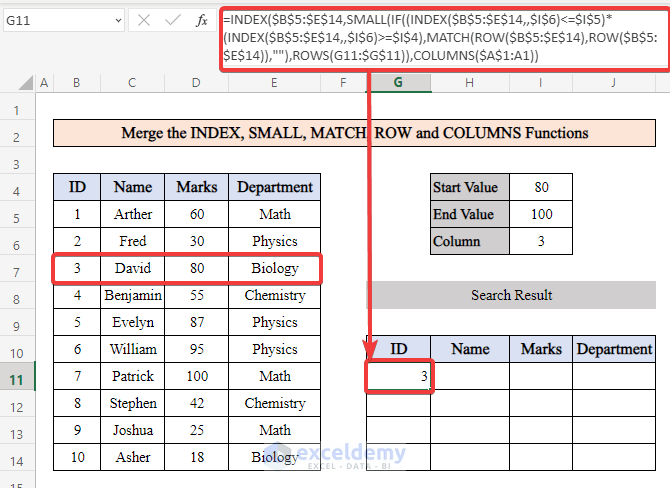
• Select cell G11 for the result.
• Enter the following formula:

INDEX($B$5:$E$14,,$I$6)= This part usually returns a single value or an entire column or row from a given cell range.

INDEX($B$5:$E$14,,$I$6)<=$I$5 = this section entered 100 as the end value.

INDEX($B$5:$E$14,,$I$6)>=$I$4 = this part entered 80 as starting value.

• Press Ctrl + Shift + Enter simultaneously to apply this formula.

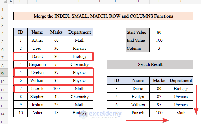
• Drag the fill handle to the right to fill the row, then down.

Read More: How to Extract Specific Data from a Cell in Excel

Things to Remember

• As the range of the data table array to search for the value is fixed, don’t forget to put the absolute reference ($) sign in front of the cell reference number to avoid the error.
• The FILTER function is only available in Excel 365. You won’t be able to use it if you are using other versions of MS Excel.
• When you are applying an array formula, you have to press Ctrl + Shift + Enter simultaneously to apply the formula.

Download the Practice Workbook

Related Articles

• Excel Formula to Get First 3 Characters from a Cell
• How to Extract Month and Day from Date in Excel
• How to Extract Month from Date in Excel
• How to Extract Year from Date in Excel
• How to Extract Data from Excel Sheet

<< Go Back To Extract Data Excel | Learn Excel