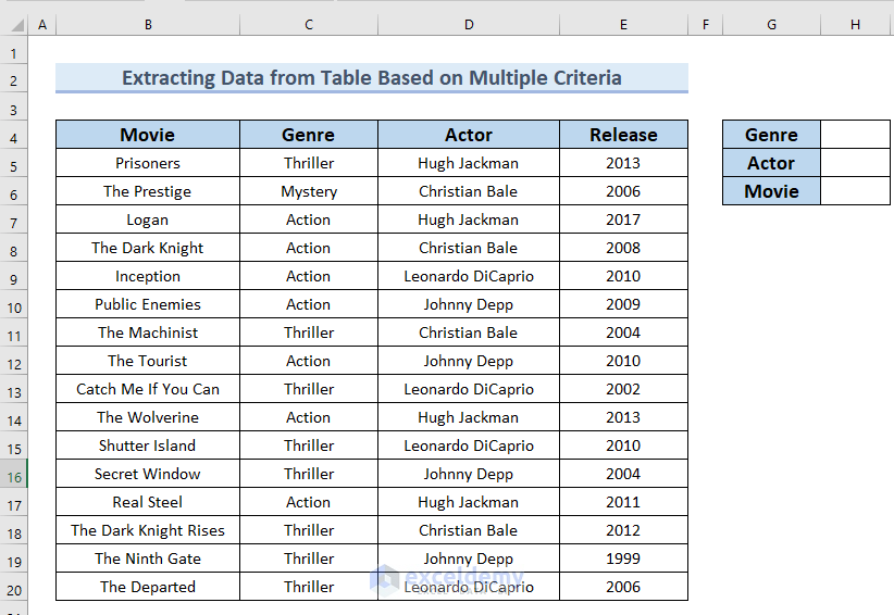
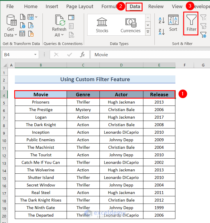
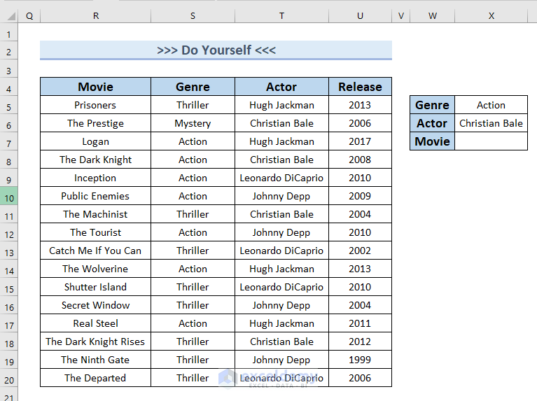
We have a dataset of movies, their genres, leading actors, and years of release.

We will provide the Genre and Actor name as criteria in a separate table and extract the Movie name.
Method 1 – Extracting a Single Value Based on Multiple Criteria
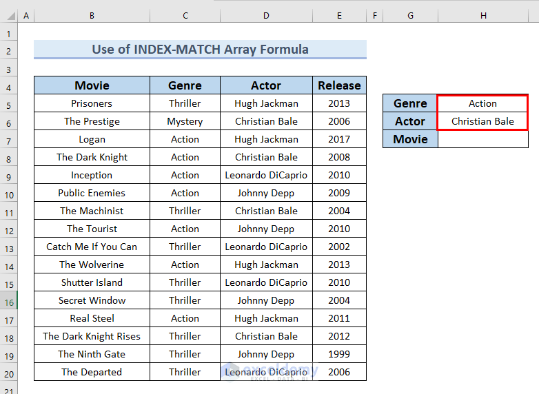
Case 1 – Using an INDEX-MATCH Array Formula
We put Action as Genre and Christian Bale as Actor.
Steps:
- Insert the following formula in cell H7.
=INDEX($B$5:$B$20,MATCH(1,($H$5=$C$5:$C$20)*($H$6=$D$5:$D$20),0))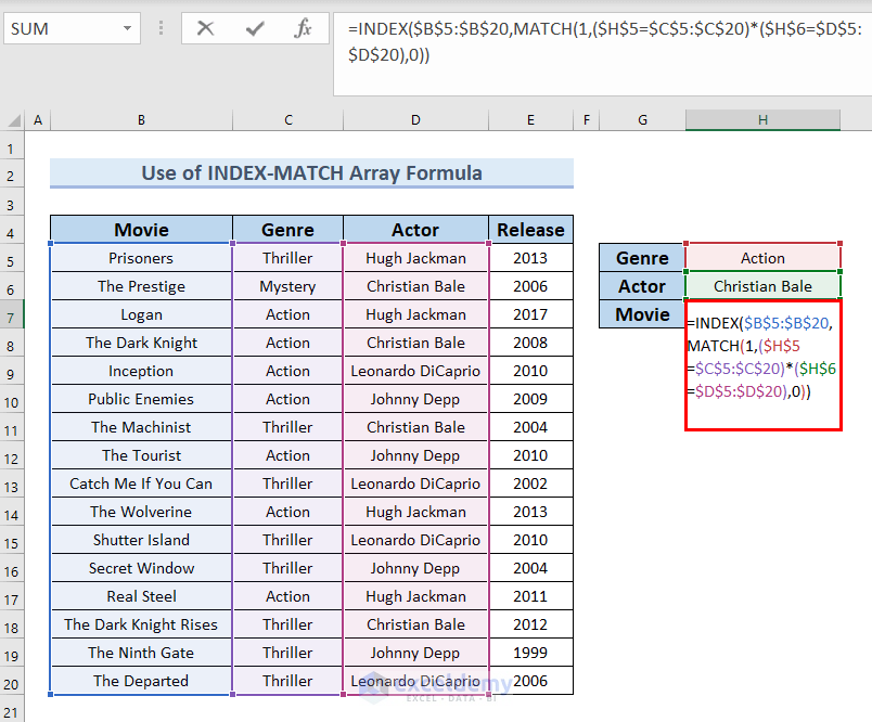
Formula Breakdown
- MATCH(1,($H$5=$C$5:$C$20)*($H$6=$D$5:$D$20),0) → the MATCH function locates the position of a lookup value in a range.
- Output: 4
- INDEX($B$5:$B$20,MATCH(1,($H$5=$C$5:$C$20)*($H$6=$D$5:$D$20),0)) →the INDEX function returns the value at a given location in a range
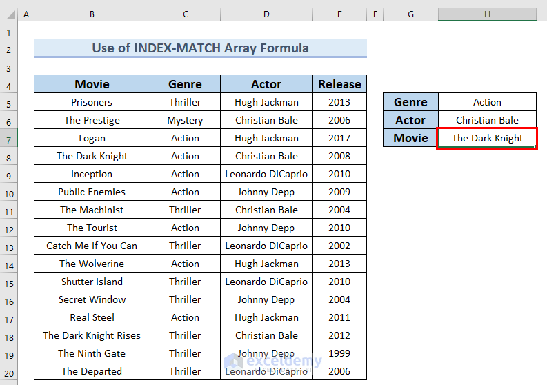
- Output: The Dark Knight
- Explanation: The Dark Knight is the Movie based on the Genre and Actor.
- Since this is an array formula, press Ctrl + Shift + Enter to apply it if you do not have Excel 365. Otherwise, press Enter.
- Change the criteria values, and you will find updated values.
Read More: How to Extract Specific Data from a Cell in Excel
Case 2 – Using an INDEX-MATCH Non-Array Formula
Steps:
- Insert the following formula in cell H7.
=INDEX($B$5:$B$20,MATCH(1,INDEX(($H$5=$C$5:$C$20)*($H$6=$D$5:$D$20),0,1),0))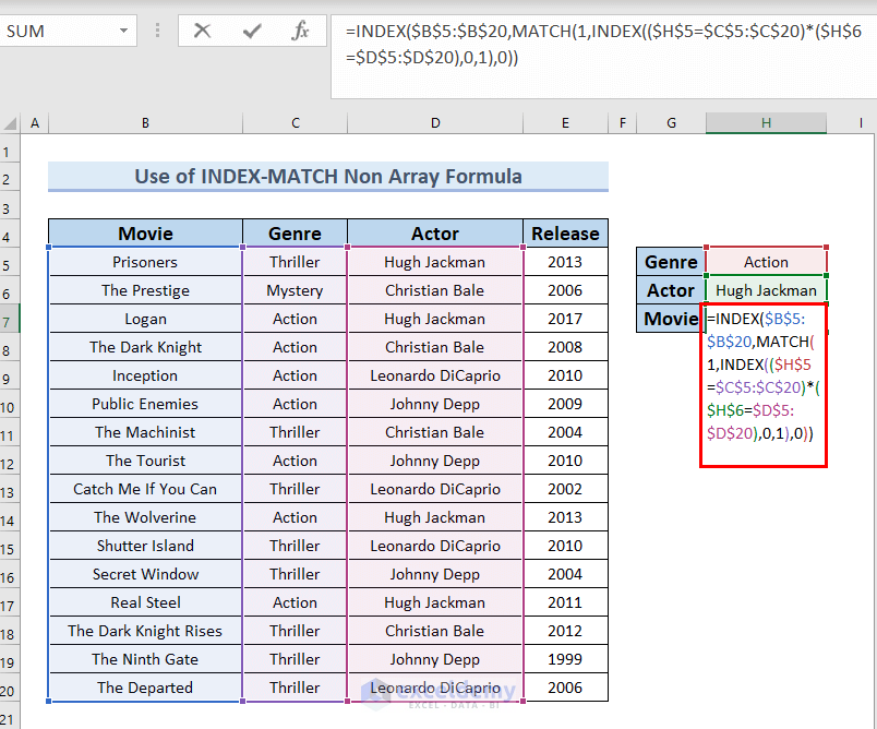
Formula Breakdown
- The MATCH function locates the position of a lookup value in a range.
- The INDEX function returns the value at a given location in a range
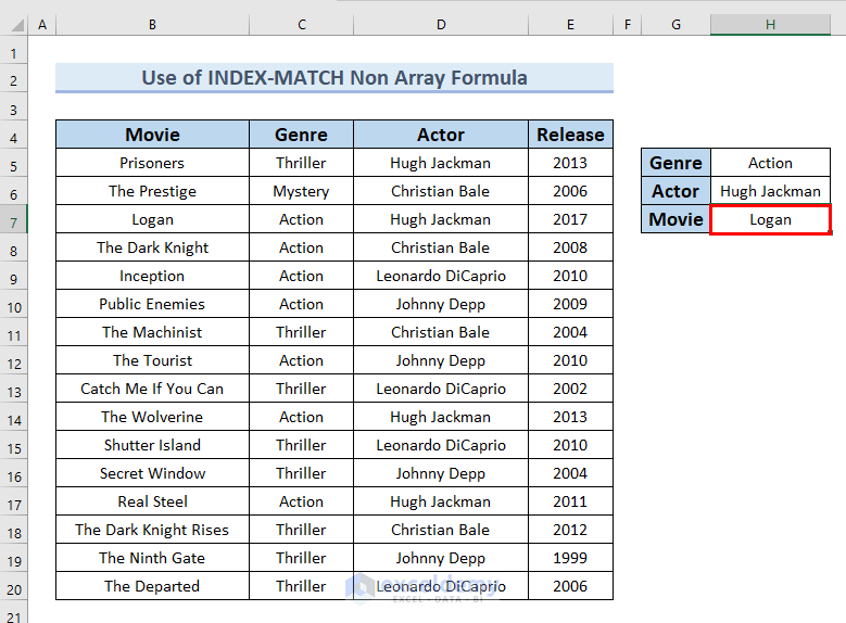
- Output: Logan
- Explanation: Logan is the Movie based on the Genre and Actor.
- Hit Enter.
- Feel free to modify the criteria values.
Read More: How to Extract Data Based on Criteria from Excel
Case 3 – Applying an INDEX-MATCH-IF Combination
Steps:
- Insert the following formula in cell H7.
=INDEX($B$5:$B$20,MATCH(1,IF($C$5:$C$20=$H$5,IF($D$5:$D$20=$H$6,1)),0))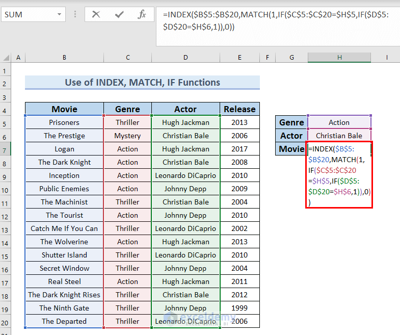
Formula Breakdown
- The MATCH function locates the position of a lookup value in a range.
- The INDEX function returns the value at a given location in a range
- The IF function makes a logical comparison between a value and the value we expect.
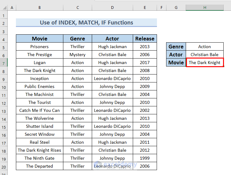
- Output: The Dark Knight
- Explanation: The Dark Knight is the Movie based on the Genre and Actor.
- Since this is an array formula, press Ctrl + Shift + Enter to apply it if you do not have Excel 365. Otherwise, press Enter.
Read More: How to Extract Data from Excel Sheet
Case 4 – Use the LOOKUP Function
The LOOKUP function performs a matching lookup in a range and returns the corresponding value. It’s a slightly obsolete function that is not recommended for large datasets.
Steps:
- Insert the following formula in cell H7.
=LOOKUP(1,1/($C$5:$C$20=$H$5)/($D$5:$D$20=$H$6),($B$5:$B$20))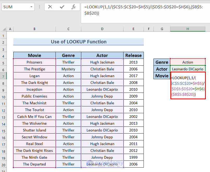
Formula Breakdown
- LOOKUP(1,1/($C$5:$C$20=$H$5)/($D$5:$D$20=$H$6),($B$5:$B$20)) → the LOOKUP function is used to search in a single row and single column.
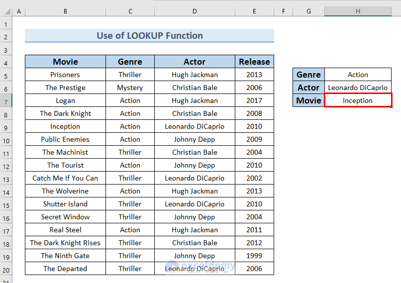
- Output: Inception
- Explanation: Inception is the Movie based on the Genre and Actor.
- Press Enter.
- Change the criteria value to see whether the formula works for other values.
Method 2 – Extracting Multiple Values Based on the Criteria
Case 1 – Using the INDEX-SMALL Combination
Steps:
- Make sure the dataset starts with row 1.
- Insert the following formula in cell H4.
=IFERROR(INDEX($B$2:$B$17,SMALL(IF(($C$2:$C$17=$H$2)*($D$2:$D$17=$H$3), ROW($B$2:$B$17)),ROW(1:1))-1,1),"")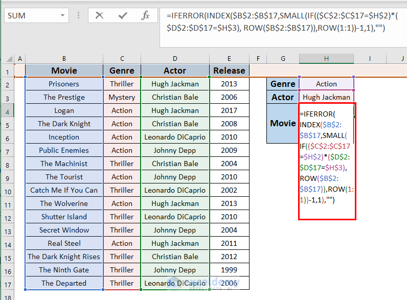
Formula Breakdown
- The INDEX function returns the value at a given location in a range
- The ROW function gets the row number of defined cells.
- The SMALL function output the K-th tiniest value in a cell range.
- The IFERROR function returns a black cell if there is any error in the formula.
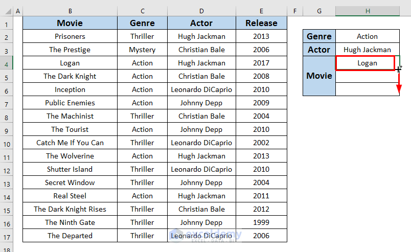
- Output: Logan.
- Explanation: Logan is the Movie based on the Genre and Actor.
- Hit Enter.
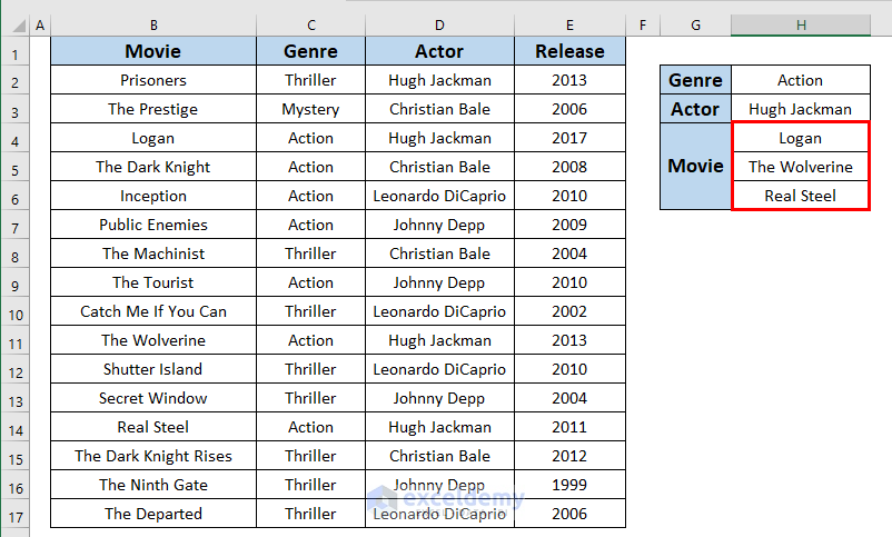
- Drag down the formula with the Fill Handle tool.
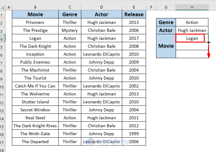
- You can see the multiple outcomes in cells H4, H5, and H6.

Read More: How to Extract Data from a List Using Excel Formula
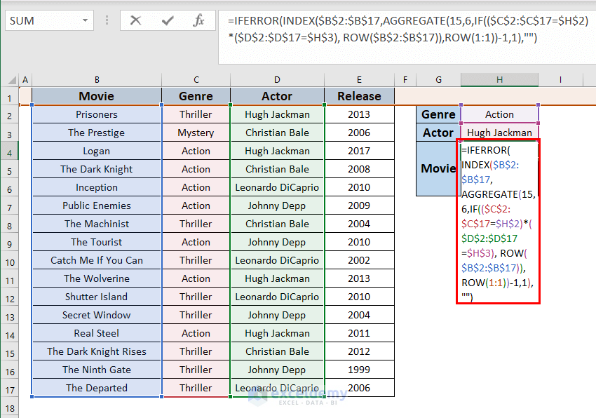
Case 2 – Applying the INDEX-AGGREGATE Combination
Steps:
- Make sure the dataset starts at row 1.
- Insert the following formula in cell H4.
=IFERROR(INDEX($B$2:$B$17,AGGREGATE(15,6,IF(($C$2:$C$17=$H$2)*($D$2:$D$17=$H$3), ROW($B$2:$B$17)),ROW(1:1))-1,1),"")
Formula Breakdown
- The INDEX function returns the value at a given location in a range
- The ROW function gets the row number of defined cells.
- The AGGREGATE function gets back an aggregate in a dataset.
- The IF function does a logical comparison between a given value and an expected value.
- The IFERROR function returns a black cell if there is any error in the formula.
- Output: Logan.
- Explanation: Logan is the Movie based on the Genre and Actor.
- Since this is an array formula, press Ctrl + Shift + Enter to apply it if you do not have Excel 365. Otherwise, press Enter.
- Drag down the formula with the Fill Handle tool.
- You can see the multiple outcomes in cells H4, H5, and H6.
Case 3 – Applying the INDEX-MATCH-COUNTIF Combination
Steps:
- Insert the following formula in cell H7.
=IFERROR(INDEX($B$5:$B$20,MATCH(0,COUNTIF(H6:$H$6,$B$5:$B$20)+IF($C$5:$C$20<>$H$5,1,0)+IF($D$5:$D$20<>$H$6,1,0),0)),"")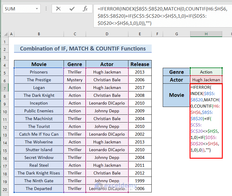
Formula Breakdown
- The INDEX function returns the value at a given location in a range.
- The COUNTIF function counts cells in a range that meets a single condition.
- The IFERROR function returns black cell if there is any error in the formula.
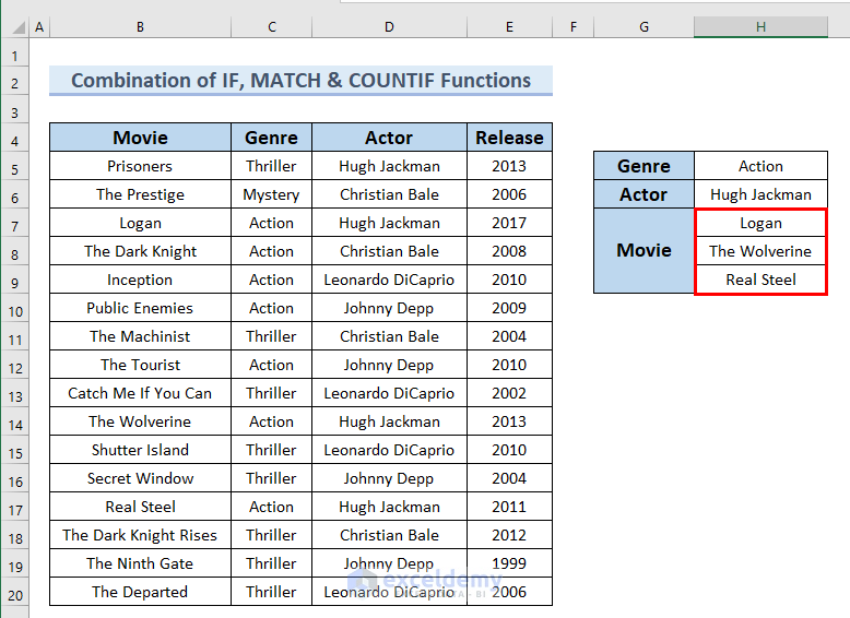
- Output: Logan.
- Explanation: Logan is the Movie based on the Genre and Actor.
- Hit Enter.
- Drag down the formula with the Fill Handle tool.
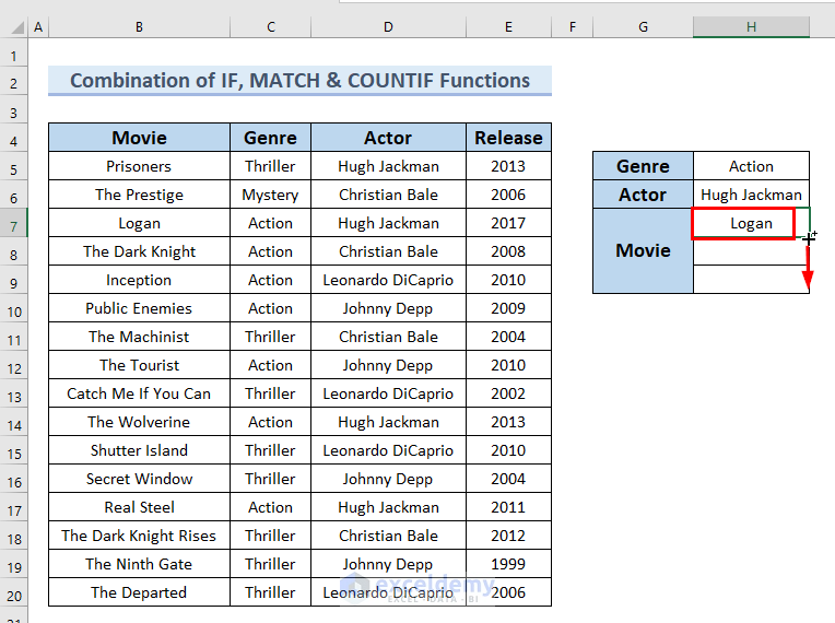
- You can see the multiple outcomes in cells H7, H8, and H9.
Read More: How to Extract Data from Cell in Excel
Case 4 – Using FILTER Function
This function is only available in Excel 365 and newer versions of Excel.
Steps:
- Insert the following formula in cell H7.
=FILTER(B5:B20,(H5=C5:C20)*(H6=D5:D20))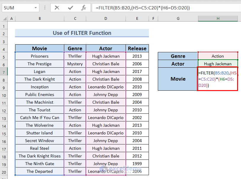
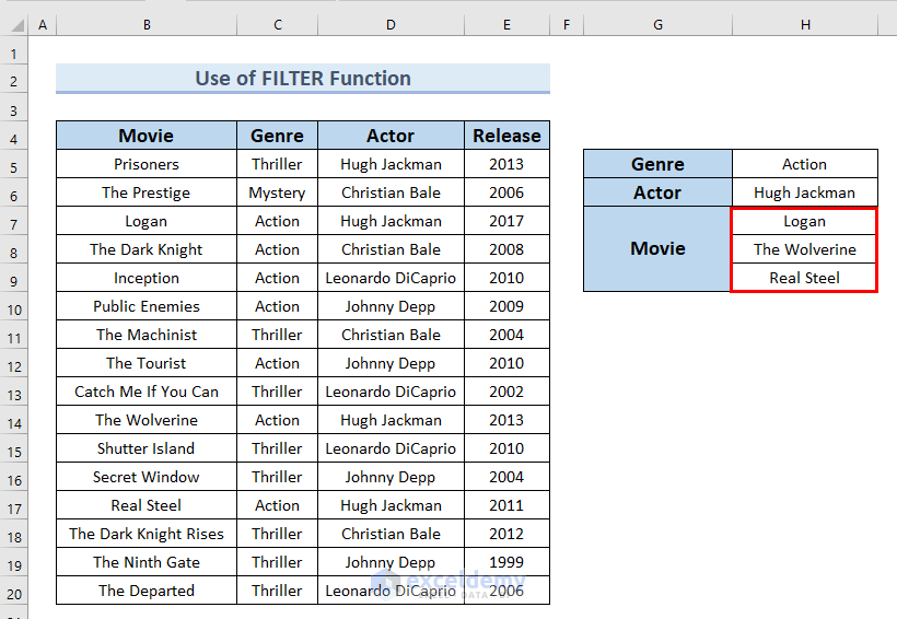
- Hit Enter.
- You can see the multiple outcomes in cells H7, H8, and H9.
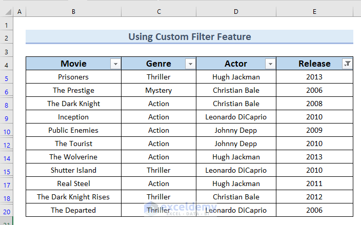
Method 3 – Use the Custom Filter Feature
We will extract the movies that have been released between 2006 and 2013.
Steps:
- Select only the headers of the dataset.
- Go to the Data tab and select Filter.
- You can see a drop-down button in each header name of the dataset.
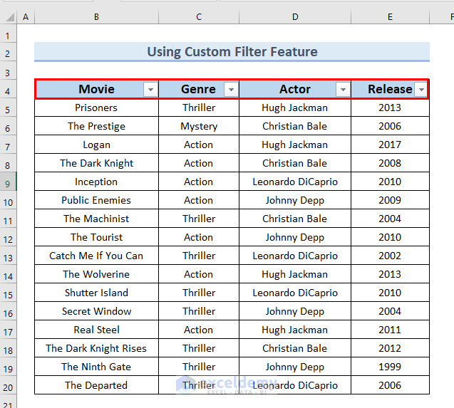
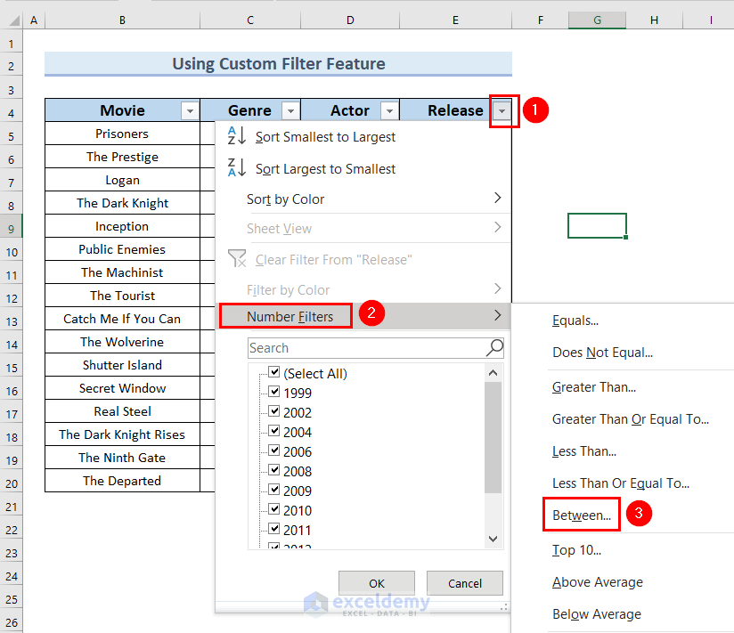
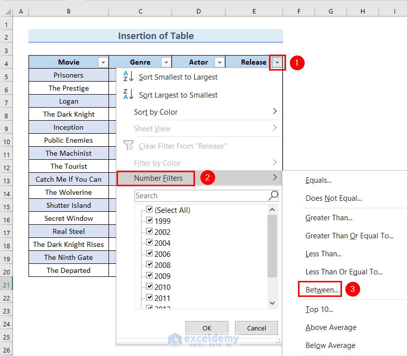
- Click on the drop-down button next to the Release column.
- Select Number Filters and choose Between.
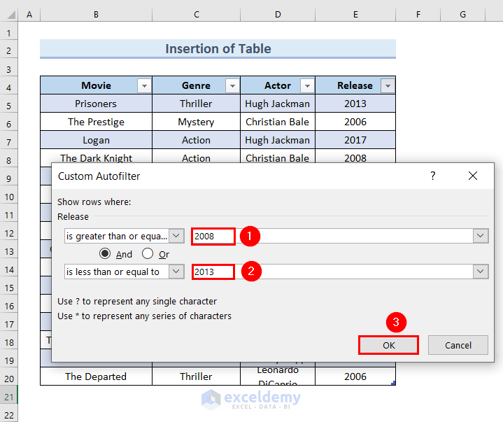
- A Custom AutoFilter dialog box will pop up.
- Type 2006 in the greater than or equal to box.
- Type 2013 in the less than or equal to box.
- Click OK.
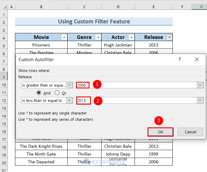
- You will get all the details for movies that were released between these years.
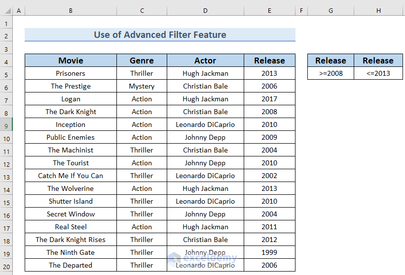
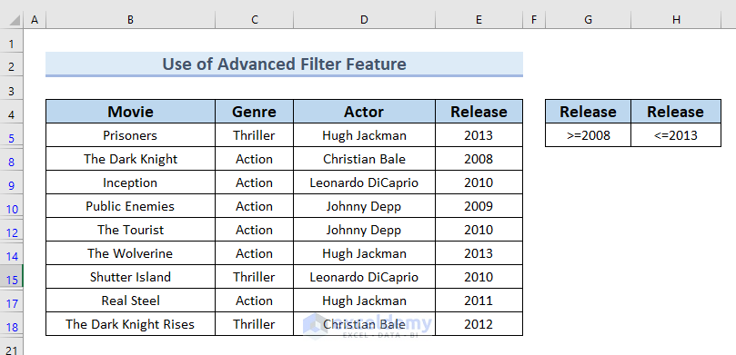
Method 4 – Apply the Advanced Filter Feature
To utilize the Advanced Filter option in Excel, you have to define the condition in your worksheet to use later. We define our condition of extracting movie details of Release year in cells G5 and H5. We typed >=2007 in cell G5 and <=2013 in cell H5. We will be using the cell reference numbers of those cells.
Steps:
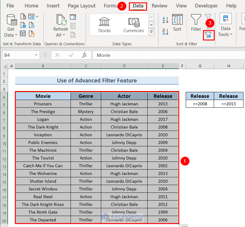
- Select the whole data table.
- From the Data tab select Advanced in the Sort & Filter group.
- An Advanced Filter dialog box will appear.
- You will see the range of your selected data in the box next to the List range option.
- In the box for the Criteria range, select the cells carrying the defined conditions. We selected cells G4:H5.
- Click OK.
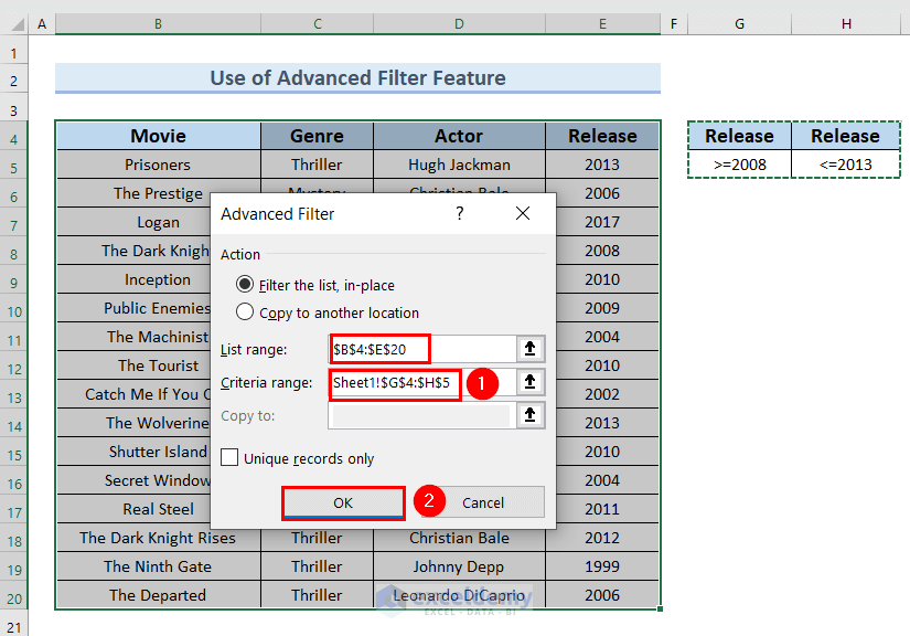
- You will get all the details only for the movies that were released between 2008 to 2013.
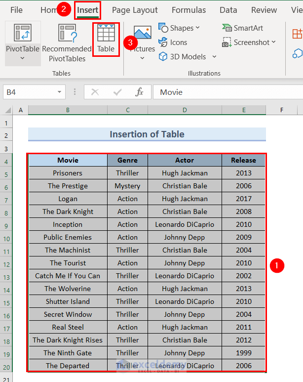
Method 5 – Insert a Table to Extract Data Based on Criteria
We will extract the movies released between 2008 and 2013.
Steps:
- Select the cells B4:E20.
- Go to the Insert tab and select Table.
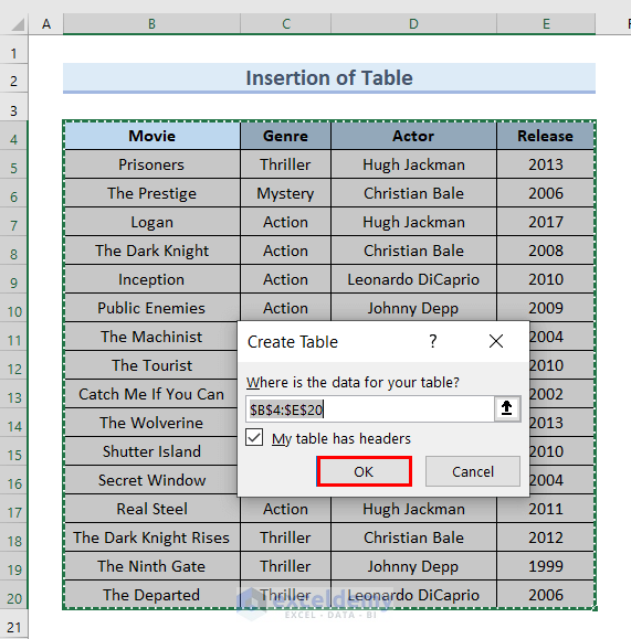
- A Create Table dialog box will appear.
- Make sure My table has headers is marked.
- Click OK.
- The headers of the Table have drop-down icons.
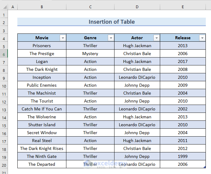
- Click on the drop-down button next to the Release column.
- From the drop-down list, select Number Filters and choose Between.
- A Custom AutoFilter dialog box will pop up.
- Type 2008 in the greater than or equal to box.
- Type 2013 in the less than or equal to box.
- Click OK.
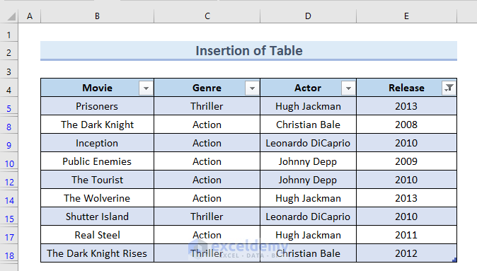
- You will get all the details only for the movies that were released between 2008 to 2013.
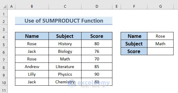
Method 6 – Apply the SUMPRODUCT Function for Numerical Values
We have a new dataset with the Name, Subject, and Score columns. You can see the criteria where we will find the Score in cell G6 for the name Rose, and for the subject Math.
Steps:
- Insert the following formula in cell G6.
=SUMPRODUCT((B5:B10=G4)*(C5:C10=G5)*(D5:D10))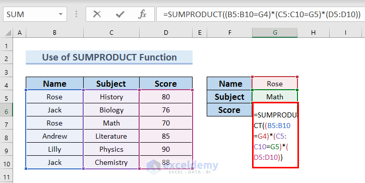
Formula Breakdown
- SUMPRODUCT((B5:B10=G4)*(C5:C10=G5)*(D5:D10)) → the SUMPRODUCT function gives the result of the sum of the values corresponding to an array.
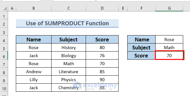
- Output: 70
- Explanation: Here, 70 is the score for Rose in Math.
- Hit Enter.
Method 7 – Use the SUM Function for Numerical Results
Steps:
- Insert the following formula in cell G6.
=SUM((B5:B10=G4)*(C5:C10=G5)*(D5:D10))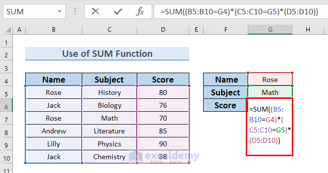
Formula Breakdown
- SUM((B5:B10=G4)*(C5:C10=G5)*(D5:D10)) → the SUM function adds the values in a range of cells.
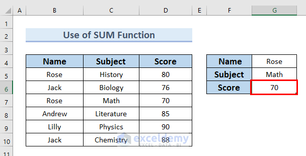
- Output: 70
- Explanation: Here, 70 is the score for Rose in Math.
- Hit Enter.
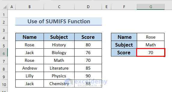
Method 8 – Use the SUMIFS Function for Finding Numerical Values
Steps:
- Insert the following formula in cell G6.
=SUMIFS(D5:D10,B5:B10,G4,C5:C10,G5) 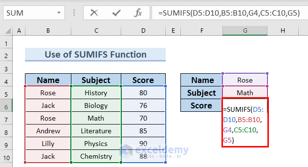
Formula Breakdown
- SUMIFS(D5:D10,B5:B10,G4,C5:C10,G5) → the SUMIFS function sums up the values that meet the given criteria.
- Output: 70
- Explanation: Here, 70 is the score for Rose in Math.
- Hit Enter.
Practice Section
We’ve included practice datasets you can use to test these methods.
Download the Practice Workbook
Extract Data from Table Based on Multiple Criteria.xlsx
Further Readings
- Excel Formula to Get First 3 Characters from a Cell
- How to Extract Month and Day from Date in Excel
- How to Extract Month from Date in Excel
- How to Extract Year from Date in Excel
<< Go Back To Extract Data Excel | Learn Excel
Get FREE Advanced Excel Exercises with Solutions!
