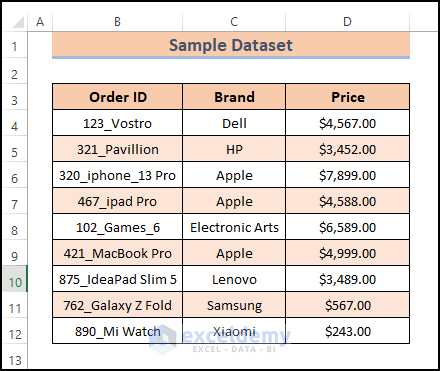
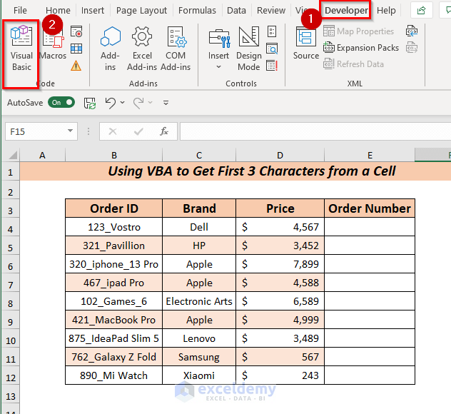
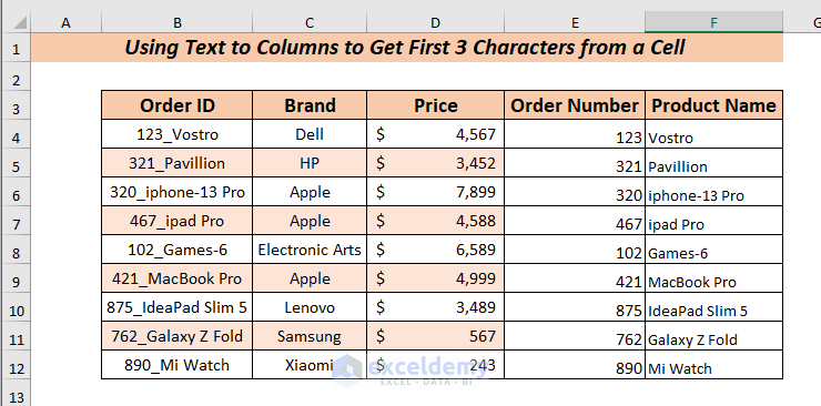
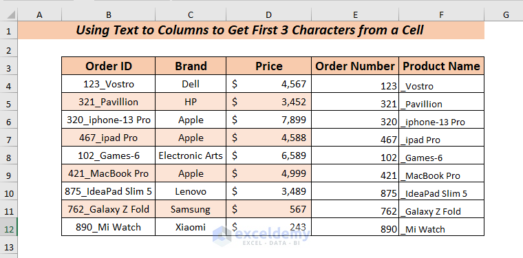
Below is a dataset of the order information for a particular product. There are 3 columns: Order ID, Brand, and Price.

Note: Use the Excel 365 edition to avoid compatibility issues.
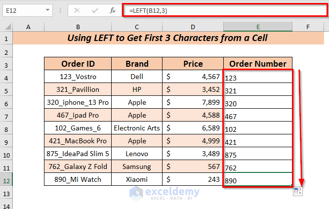
Method 1 – Using the LEFT Function to Get the First 3 Characters from a Cell
STEPS:
- Select cell E4.
- Enter the following formula in the Formula Bar:
=LEFT(B4,3)- In the LEFT function, I selected cell B4 as text and the num_chars 3. The first 3 characters from the left will be extracted.
- Press ENTER.
- You will see the extracted 3 characters in the Order Number column.
- You can use the Fill Handle to AutoFill the formula in the rest of the cells.
Read More: How to Extract Data from Excel Sheet
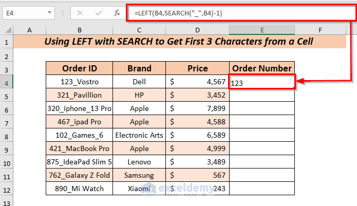
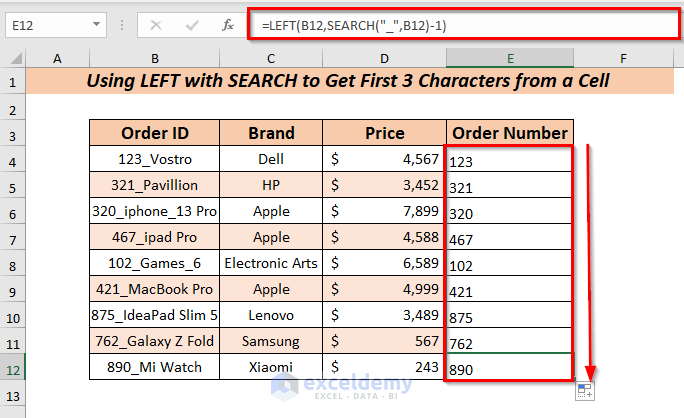
Method 2 – Applying LEFT with the SEARCH Function to Extract the First 3 Characters
STEPS:
- Select cell E4.
- Enter the following formula in the selected cell or Formula Bar.
=LEFT(B4,SEARCH("_",B4)-1)- In the SEARCH function, given (_) in find_text, then within_text, I selected cell B4. The SEARCH function will give the position number of the given text, and then 1 will be subtracted from the position. It will work as num_chars for LEFT. The LEFT function will extract the characters from the left.
- Press ENTER.
You will see the extracted 3 characters in the Order Number column.
- Use the Fill Handle to AutoFill the formula in the other cells.
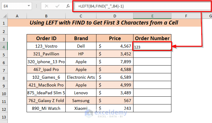
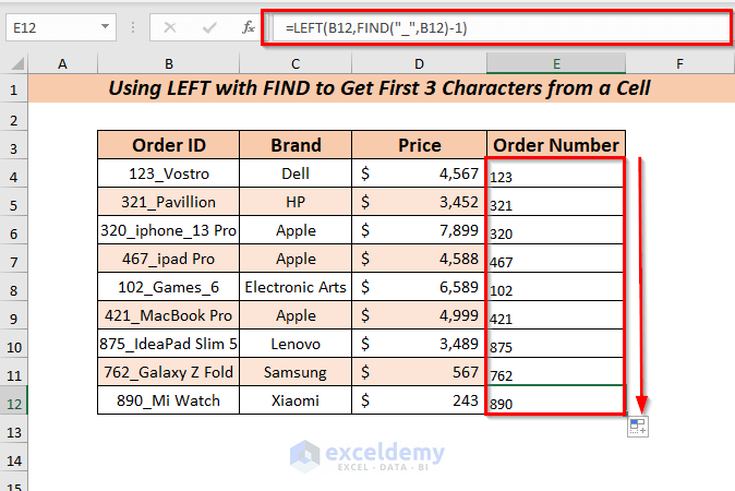
You can also use the LEFT function with the FIND function to get the first 3 characters from the left if you want to extract value from a particular text and a special character.
STEPS:
- Select cell E4.
- Enter the following formula in the selected cell or Formula Bar:
=LEFT(B4,FIND("_",B4)-1)- In the FIND function, given (_) in find_text, then within_text, I selected cell B4. The FIND function will show the position number of the given text, and then 1 will be subtracted from the position. It will work as num_chars for LEFT. The LEFT function will extract the characters from the left.
- Press ENTER.
- You will see the extracted 3 characters in the Order Number column.
- Use the Fill Handle to AutoFill the formula in the other cells.
Read More: How to Extract Data from Cell in Excel
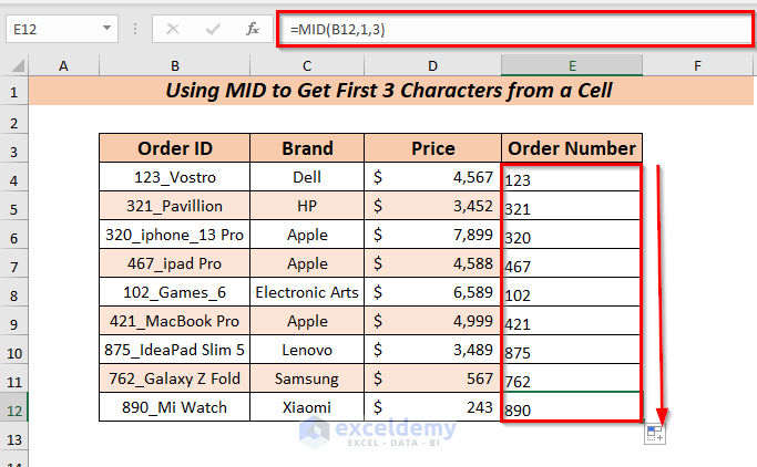
Method 3 – Applying the MID Function for the First 3 Characters From a Cell
STEPS:
- Select cell
- Enter the following formula in the selected cell or Formula Bar:
=MID(B4,1,3)- In the MID function, I selected cell B4 as text, start_num 1, and num_chars 3. The MID function will extract the characters starting from the 1st character to the 3rd character.
- Press ENTER.
- You will see the extracted 3 characters in the Order Number column.
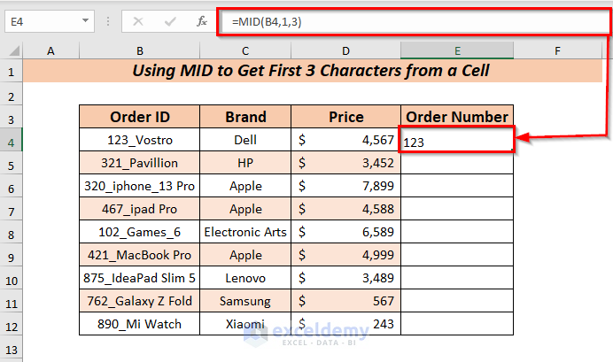
- Use the Fill Handle to AutoFill the formula in the other cells.
Read More: How to Extract Data from a List Using Excel Formula
Method 4 – Getting the First 3 Characters from a Cell Through Excel VBA
STEPS:
- Open the Developer tab >> select Visual Basic.
- It will open a new window of Microsoft Visual Basic for Applications.
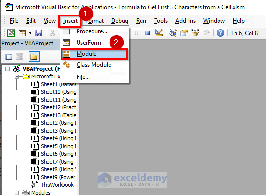
- Go to Insert >> select Module.
- Enter the code in the Module.
Sub Get_First_3Character()
Dim R As Integer
For R = 4 To 12
   ActiveSheet.Cells(R, 5).Value = Left(Cells(R, 2), 3)
Next R
End Sub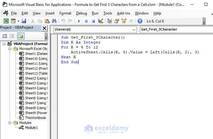
- Here R represents the row numbers.
- In the LEFT function the num_chars = 3.
- Used a For loop to continue the process for the row range.
- Save the code and go back to the worksheet.
- Select cell C6.
- Open the View tab >> from Macros >> select View Macro.
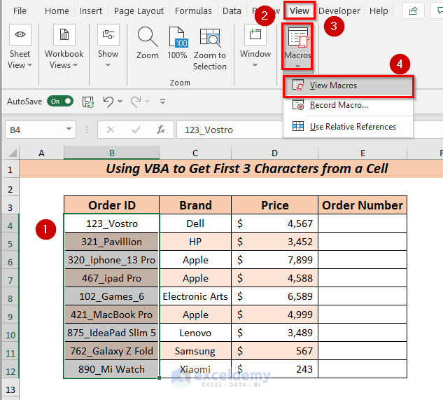
- A dialog box will pop up. Select the Macro to Run.
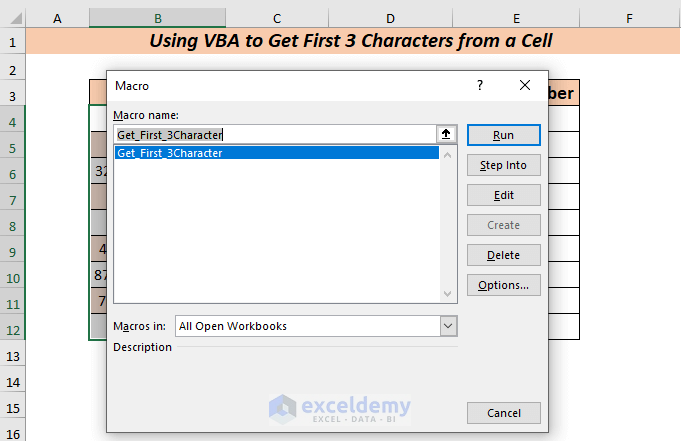
- From the dialog box select the Macro name Get_First_3Character.
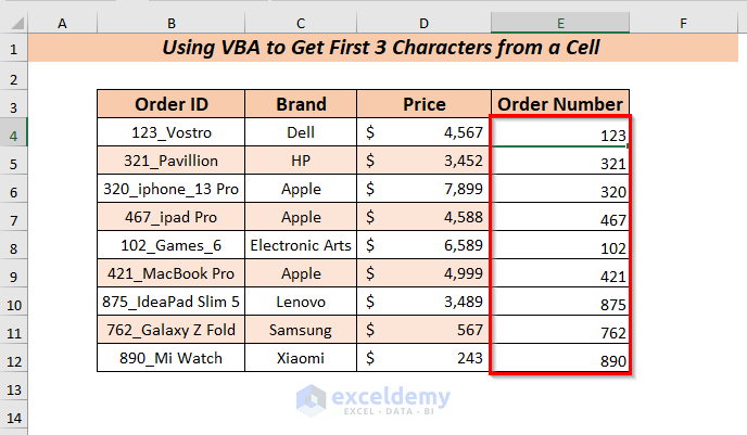
- You will see the character from the used row range in VBA is extracted in the column.
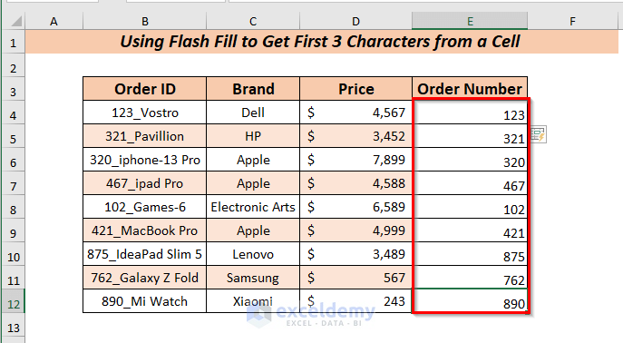
Method 5 – Utilizing Flash Fill to Return the First 3 Characters from a Cell
STEPS:
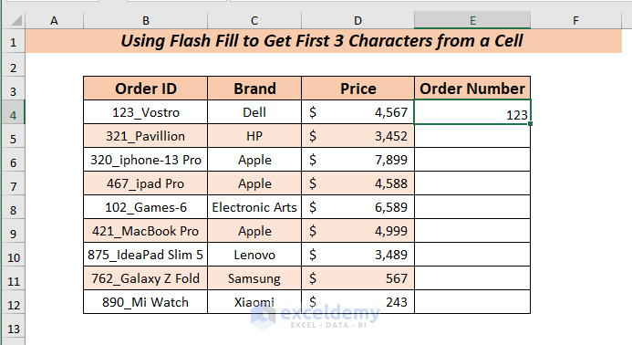
- Enter the pattern of the first 3 characters from cell B4.
- Open the Data tab >> from Data Tools >> select Flash Fill.
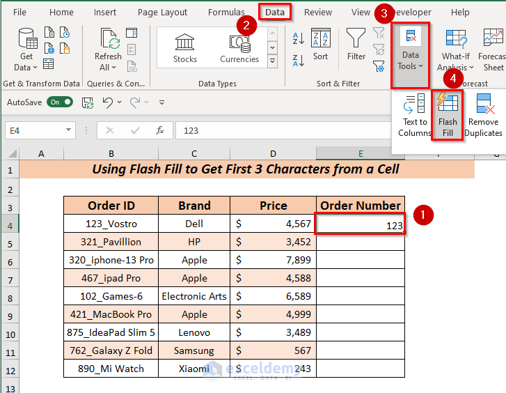
- All the remaining cells of the Order Number will be filled with 3 characters from the Order ID column.
Read More: How to Extract Specific Data from a Cell in Excel
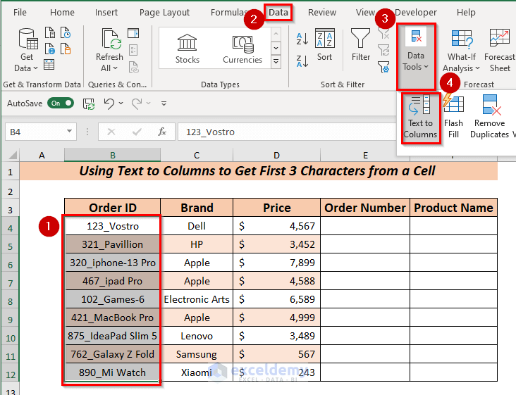
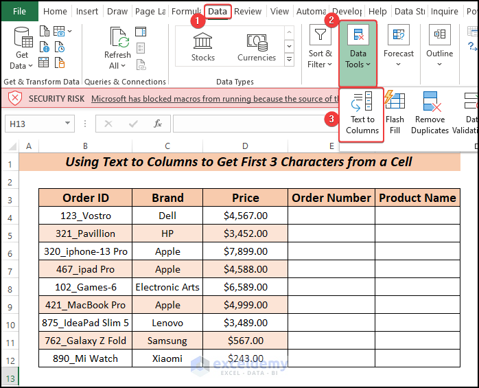
Method 6 – Extracting the First 3 Characters from a Cell with the Text to Columns Feature
a) Using Delimited
STEPS:
- Select the B4:B12 cell range to split
- Open the Data tab >> from Data Tools >> select Text to Columns.
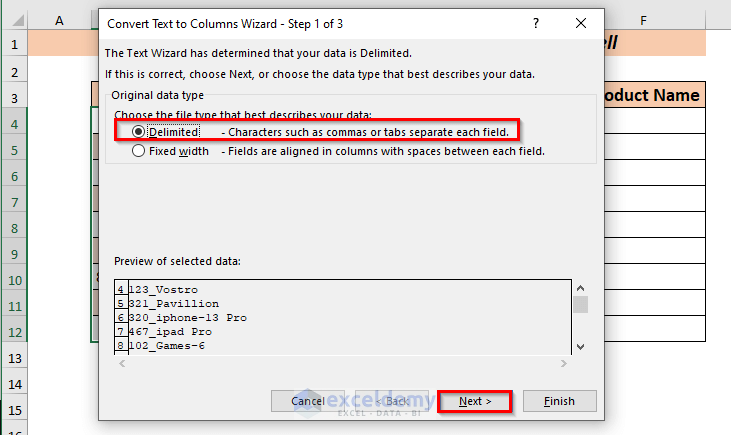
- A dialog box will pop up. Select the file type Delimited and click Next.
- In the dialog box select the Delimiters your value has.
- Click Next.
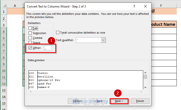
- In the dialog box select the Delimiters your value has.
- Click Next.
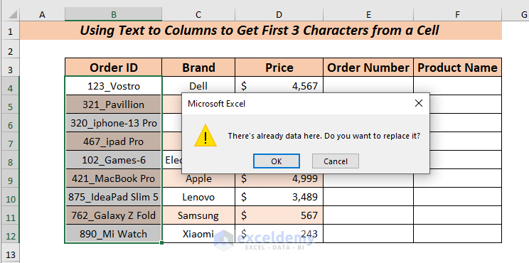
- A warning message will pop up. Click OK.
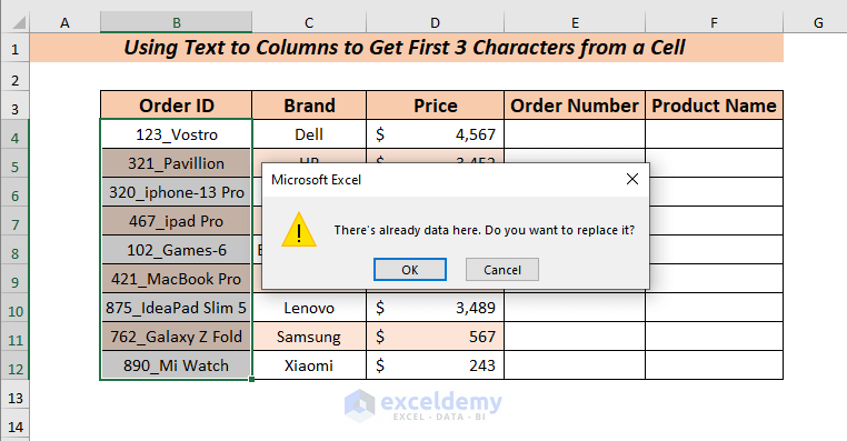
- You will see the first 3 characters in the Order Number column.
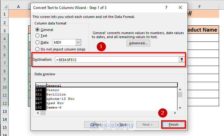
b) Using Fixed Width
STEPS:
- Select the cell or range of cells that you want to split.
- Open the Data tab >> from Data Tools >> select Text to Columns.
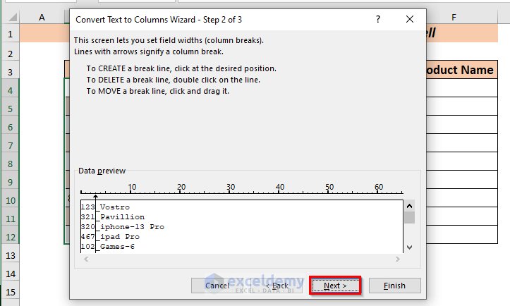
- A dialog box will pop up. Select the file type Fixed Width and click Next.
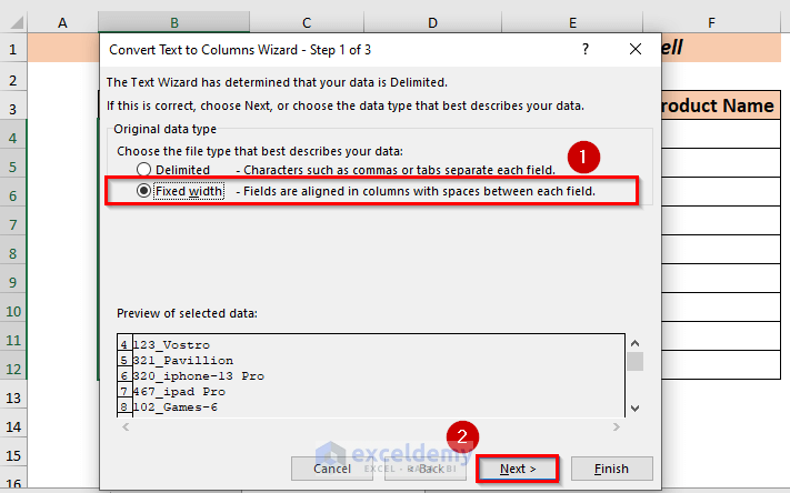
- In the dialog box create a break in the line. To do that, click on the desired position.
- Click Next.
- You can choose the Destination or keep it as is.
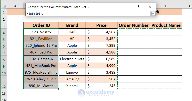
- Click Finish.
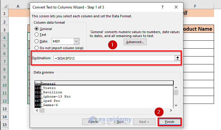
- A warning message will pop up. Click OK.
- You will see the first 3 characters in the Order Number column.
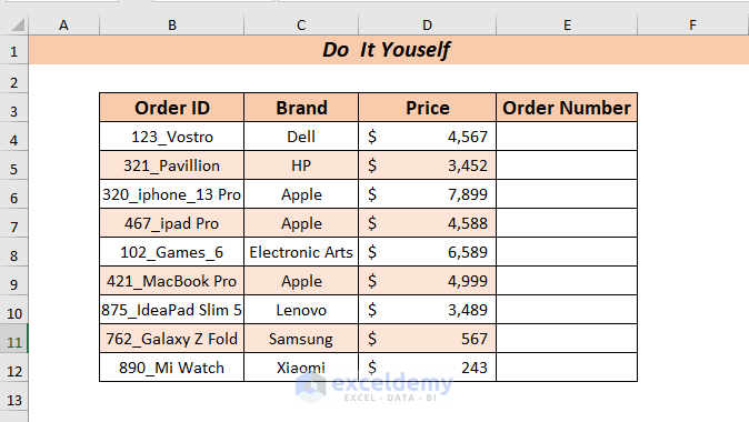
Practice Section
Here’s a practice sheet you can use to practice these methods:
Download to Practice
Related Articles
- How to Extract Month and Day from Date in Excel
- How to Extract Month from Date in Excel
- How to Extract Year from Date in Excel
- How to Extract Data Based on Criteria from Excel
- How to Extract Data From Table Based on Multiple Criteria in Excel
<< Go Back To Extract Data Excel | Learn Excel
Get FREE Advanced Excel Exercises with Solutions!
