Method 1 – Combining INDEX and MATCH Functions
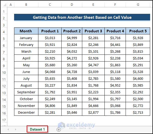
We have a dataset that includes several months and the sales amount of several products. We’ll get the data in another sheet.
Steps
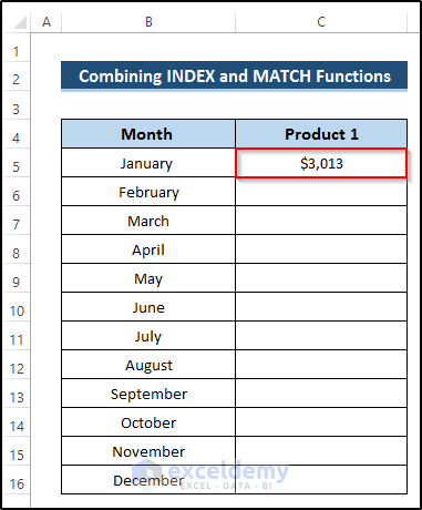
- Make a new sheet.
- Insert the month names in the new sheet in column B (B5:B16).
- Select cell C5.
- Insert the following formula.
=INDEX('Dataset 1'!C5:G5,MATCH('Dataset 1'!C5,'Dataset 1'!C5:G5,0))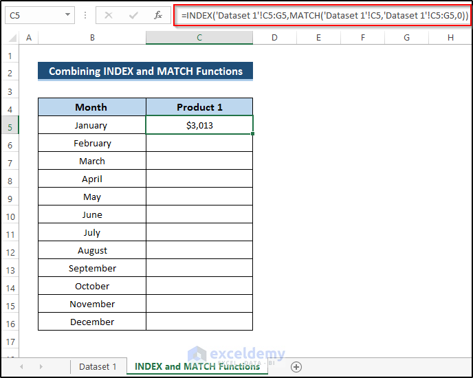
- Press Enter to apply the formula.
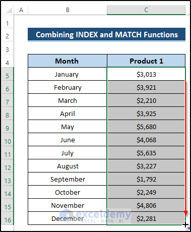
- Drag the Fill Handle icon down the column.
Breakdown of the Formula
INDEX(‘Dataset 1’!C5:G5,MATCH(‘Dataset 1′!C5,’Dataset 1’!C5:G5,0)): The MATCH function in Excel is used to locate the position of a lookup value in a row, column, or table. Here, cell C5 is the lookup value and the range of cells C5 to G5 defines the lookup array. Finally, the MATCH function finds the exact match of a value from the array of another sheet. Then, this returned value will act as an input value of the INDEX function. The INDEX function returns that value from the given array.
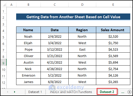
Method 2 – Using the VLOOKUP Function
We have a sales dataset and will fetch the sales for a salesperson in a different worksheet.
Steps
- Make a new worksheet where you want to apply the VLOOKUP function.
- Insert the salespeople’s names in column B (B5:B12).
- Select cell C5.
- Insert the following formula.
=VLOOKUP(B5,'Dataset 2'!$B$4:$E$12,4,0)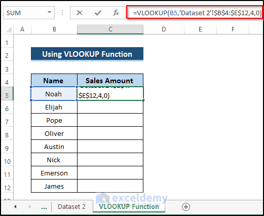
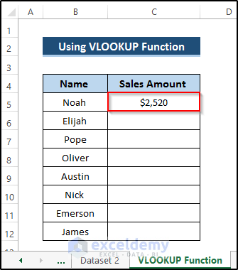
- Press Enter to apply the formula.
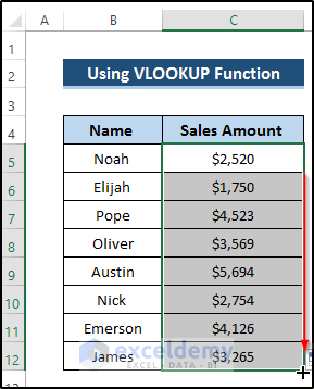
- Drag the Fill Handle icon down the column.
Breakdown of the Formula
VLOOKUP(B5,’Dataset 2′!$B$4:$E$12,4,0): The VLOOKUP function takes the lookup value and finds the required value using the given lookup array and column number. Here, cell B5 means Noah which is the lookup value. Then, we provide the lookup array and column number. By using this input, the VLOOKUP function gives us the required value that appeared in column 4.
Method 3 – Applying the HLOOKUP Function
We’ll use the same sales dataset.

Steps
- Make a new worksheet where you would like to use the HLOOKUP function.
- Enter the column header which you want to extract in a cell. We would like to get the sales amount.
- Make a helper column D and fill it in with a series starting from 1.
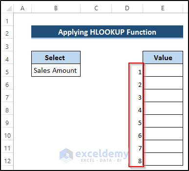
- Select cell E5.
- Insert the following formula.
=HLOOKUP($B$5,'Dataset 2'!$B$4:$E$12,D5+1,0)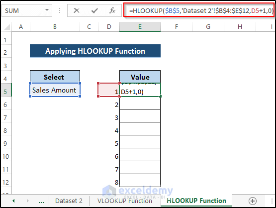
- Press Enter to apply the formula.
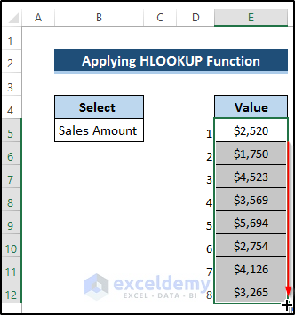
- Drag the Fill Handle icon down the column.
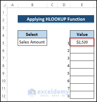
Breakdown of the Formula
HLOOKUP($B$5,’Dataset 2′!$B$4:$E$12,D5+1,0): The HLOOKUP function performs a horizontal lookup. Here, we define the lookup value and lookup array. The sales amount is the lookup value. The HLOOKUP function search this in the given array and given row number. The helping column is used to define the row number. Finally, the HLOOKUP function returns $2520 which is the sales amount for the first case.
Read More: How to Pull Data from Multiple Worksheets in Excel
Method 4 – Use the Advanced Filter
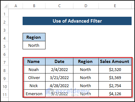
We’ll pull out the details of the salespeople who sold products in the north.

Steps
- Go to the new worksheet where you would like to put the filtered value.
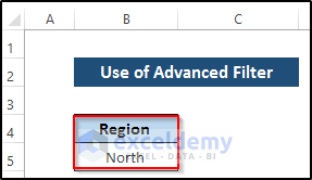
- Create a new column called Region which will be used as the criteria in the advanced filter option.
- Go to the Data tab on the ribbon.
- Select the Advanced option from the Sort & Filter group.

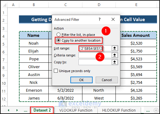
- The Advanced Filter dialog box will appear.
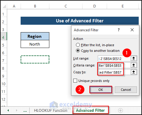
- Select Copy to another location from the Action section.
- Select the range of cells B4:E12 from the Dataset 2 worksheet.
- In the Criteria range section, select the range of cells B4 to B5 from the Advanced Filter worksheet.
- Select a place where you want to copy.
- Click on OK.
- We will get the following result.
Download the Practice Workbook
Further Readings
- Extract Filtered Data in Excel to Another Sheet
- How to Pull Values from Another Worksheet in Excel
- Pull Same Cell from Multiple Sheets into Master Column in Excel
- Extract Data from One Sheet to Another Using VBA in Excel
- How to Pull Data from Multiple Worksheets in Excel VBA
- Excel Macro: Extract Data from Multiple Excel Files
<< Go Back To Extract Data Excel | Learn Excel
Get FREE Advanced Excel Exercises with Solutions!

A very powerful message and useful presentation. Thank you for presenting this.
James, thanks for your feedback.
Glad to hear that it was useful for you.
Regards
Thank you for this useful article, nicely explained.
Thanks, Surya!
Very simple, good
Thanks, FERREIRA for your feedback!
Hi Mr. Kawser!
I find your website really amazing. I am a newbie in excel and the way you present your excel is fantastic and so easy to understand. I want to compile all of them so I can easily go through them without browsing the internet everytime. I wish you have a pdf also on this. Thanks a lot!
Hi Gilbert,
I am really sorry for not having PDF formats of the Articles.
But you can make your own PDFs. Only thing is: you can use it personally. Not for commercial use, of course.
Hope you understand.
Thanks and regards
Kawser Ahmed
Hi Kawser
Have trouble in retrieving information from 3 excel, with 3 same sheet names.
In 1 excel – sheet 3 is where formula is to go, reference by name is in column A, sheet 1 is where to retrieve information from, Column A is name, Column B is date, Column C is Distance – so on across 20 columns.
Name by latest date, 2nd latest date, & third latest date.
Name appears in sheet 1 Column A 100 times
Dates in sheet 1 Column B from top B6 = 1-01-2020 — B64000 = 5-01-2020 Month/Date/Year & adding.
Some of the Formula’s tried to retrieved from one sheet eg:
Formula =VLOOKUP(A6,RESULTS!A:A,1,FALSE)
=VLOOKUP(A6,RESULTS!A:B,2,FALSE)
=VLOOKUP($A$6,RESULTS!$A$6:$C$90000,3,4)
=MAX(A6=RESULTS!$A$6:$A$90000,RESULTS!$B$6:$B$90000,””)*FALSE
=MAX(IF(A6,RESULTS!A:A6:A90000=A6,B6:B90000)+1)
=INDEX(“RESULTS!A”,MATCH(1,(RESULTS!A=A6)*(RESULTS!A=A6)*1))
Regards
Tony
Hi Tony,
I couldn’t fully understand what you need from your comment. You said you want to retrieve information from Sheet1. But you are looking for information in the “RESULTS” sheet in all of those formulas that you’ve tried.
Can you share the workbook with us? Thanks.
Regards
Md. Shamim Reza (ExcelDemy Team)
Hey Brother
I am trying to write a function that will retrieve a cell value from another sheet on the same file using the name of the sheet identified in as a cell value in the current sheet but cant get this to work. Could you offer a solution?So the name of the sheet appears in a cell as just the name and i want to reference that name to create an address to use in a lookup function
Can you send me the Excel sheet to this email [email protected]? I will take a look at your problem.
Hey
I am looking for way to pull several cells from a large excel based on a key that exists in my sheet. in other words I am looking for a replacement to perform a vlookup for each cell for the same key. In other words I have an excel sheet with some data and would like to add data from the reference excel file to retrieve cells 15,20,45,73 into my sheet to cells F3:I3 for the key in cell A3.
Hi
I couldn’t understand the problem from your comment. Please explain what you need in details and share the workbook if possible. Then we will try our best to find you the solution.
Thanks for reaching out to us. Keep in touch.
Regards
Md. Shamim Reza (ExcelDemy Team)
Good afternoon,
I am trying to move information from worksheet1 to worksheet2 if the worksheet1 has information in it. For example if CELL A2 in worksheet2 is found in worksheet1 and has information on lines B2, C2 and D2, I want that information to be placed in worksheet2 lines B2,C2 and D2.
In worksheet1 CELL A2 through A440 have different SLOT numbers (job numbers) in them. In worksheet2 CELL A2 through A440 MAY have the same SLOT numbers and I want the information in lines B2, C2 and D2 to be brought to worksheet2.
I am not very familiar with all the functions that I know Excel has to offer. I have been trying really hard to use different functions but have found it very difficult.
This is what it looks like worksheet1
Slot # Hire Date Last Name First Name
AA001 01/01/00 DOE JOHN
AA002 02/02/00 RAY JANE
AA003 01/10/00 MI OLIVE
AA004 05/11/24 SO SON
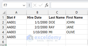
This is what it looks like in worksheet 2
Slot # Hire Date Last Name First Name
AA001
AA002
AA003
AA005
I want to move information from worksheet1 to worksheet2 if the slot # is in both worksheets.
Your help is much appreciated.
Hello Guadalupe Valdez,
To get value from another workbook you can use the VLOOKUP function.
In Worksheet2:
In cell B2 Enter the following formula:
=IFERROR(VLOOKUP($A2,[Worksheet1.xlsx]Sheet1!$A$2:$D$5, 2, FALSE), “”)
This formula looks up the Slot number in A2 of Worksheet2 in the range A2
of Worksheet1. The IFERROR function will return an empty string if no match is found.
Then, drag the formula down to A440 cell.
Use the same formula by changing the column number for First and Last name.
In cell C2 of Worksheet2, enter the following formula:
=IFERROR(VLOOKUP($A2, [Worksheet1.xlsx]Sheet1!$A$2:$D$440, 3, FALSE), “”)
In cell D2 of Worksheet2, enter the following formula:
=IFERROR(VLOOKUP($A2, [Worksheet1.xlsx]Sheet1!$A$2:$D$440, 4, FALSE), “”)
Final Output:
Here, I am attaching the Excel Files:
Worksheet1.xlsxhttps://www.exceldemy.com/wp-content/uploads/2024/06/Worksheet2.xlsx
Worksheet2.xlsx
Regards
ExcelDemy
I’m trying to use these functions but keep showing an error. I’m trying to pull 4 specific project titles from a sheet of 40 entries. Basically trying to collect data in its own summary from a large pool of data, so instead of combing through all 50, I’d like to be able to pull just those specific projects in it’s own table.
Hello Ines ,
If you’re getting errors while pulling specific project titles into a summary table, it could be due to the formula setup or data range selection. For this task, the FILTER function (available in Excel 365 and Excel Online) is very effective. You can use a formula like:
=FILTER(A2:B41, ISNUMBER(MATCH(A2:A41, {“Project1″,”Project2″,”Project3″,”Project4”}, 0)))
1. Replace A2:B41 with your actual data range.
2. Update {“Project1″,”Project2″,”Project3″,”Project4”} with your specific project titles.
If you’re not using Excel 365, you may need to use a combination of INDEX and MATCH with helper columns. Double-check your ranges and project names for typos. If you share the exact error message or formula, I can help further!
Regards
ExcelDemy