How to Pull Data from Multiple Worksheets in Excel (4 Quick Ways)

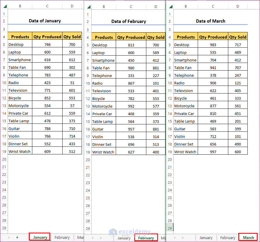
We have three worksheets in a workbook. They contain the sales records of some items over January, February and March, respectively. We’ll pull data from these three worksheets into a single worksheet to use for calculations.

Method 1 – Use a Formula to Pull Data from Multiple Worksheets

• Place the name of the sheet (Sheet_Name!) before the cell reference when there are cell references of multiple sheets in a formula.
• Let’s try to find out the total number of each product sold in the three months. The sales are in column D, starting with D5.

Steps

• Select any cell in any worksheet and apply the formula:

• Drag the Fill Handle to copy the formula to the rest of the cells.

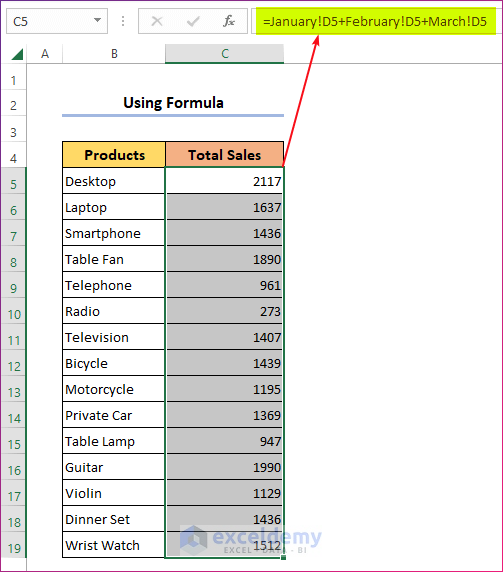
• You’ll get a sequential list of sales totals.
• Note that the formula doesn’t check whether the items in the corresponding columns match, it just pulls the numbers based on the cell reference.

Using a 3D Reference Formula:

• Alternatively, you can use the following formula if the sheets are ordered one after another in the Excel window.

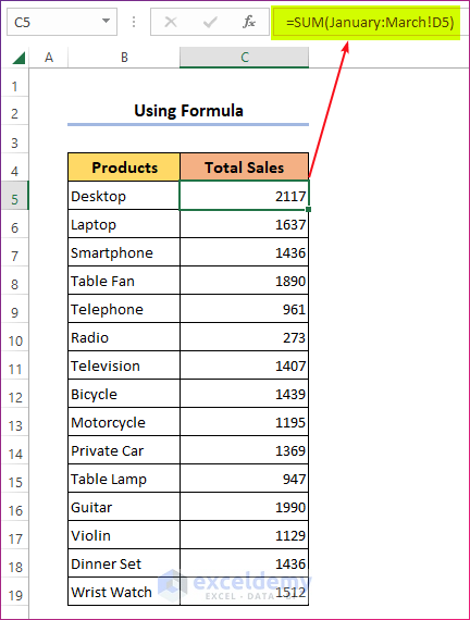
Read More: How to Pull Data from Multiple Worksheets in Excel VBA

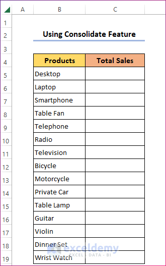
Method 2 – Pulling Data from Multiple Worksheets with the Consolidate Feature

Steps:

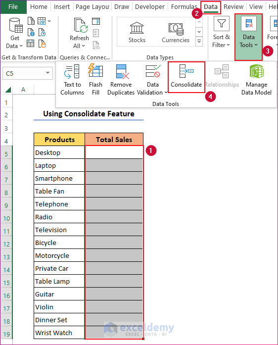
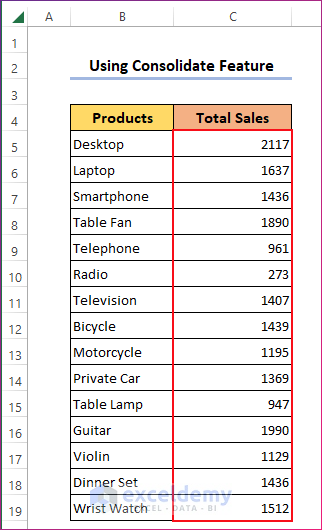
• Create a blank dataset with the product names and add a column named Total Sales. Keep the cells under this column blank.

• Select the C5:C19 range in any worksheet.
• Go to the Data tab and select Consolidate under the Data Tools section.

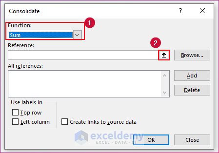
• You will get the Consolidate dialog box.
• Under the option Function, select the operation you want to perform on the data from multiple worksheets. We chose Sum.
• Click on the Import icon right to the Reference box.

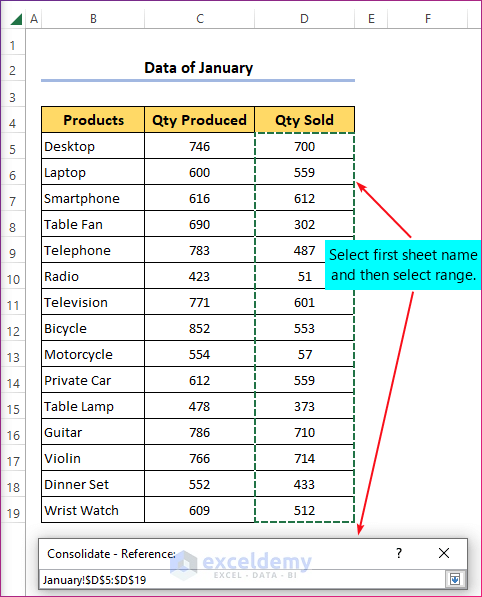
• The Consolidate box will be compressed to Consolidate – Reference. Select the desired range of cells from the first sheet.
• Click the Import icon to the right.

• You will find the cell reference of the selected range inserted in the Reference box. Click the Add button right to the Add references box.

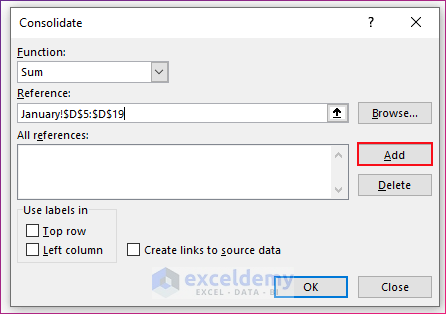
• You will find the references of the selected range inserted in the Add references box.
• Select the other ranges of cells from the other worksheets and insert them in the Add references box in the same way. For the sample, select D5:D19 from the worksheet February and D5:D19 from the worksheet March.

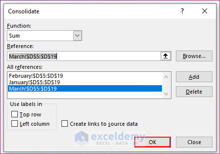
• Click OK. You will find the sum of the three selected ranges from three worksheets inserted in the empty range.

Method 3 – Using Macros to Pull Data from Multiple Worksheets

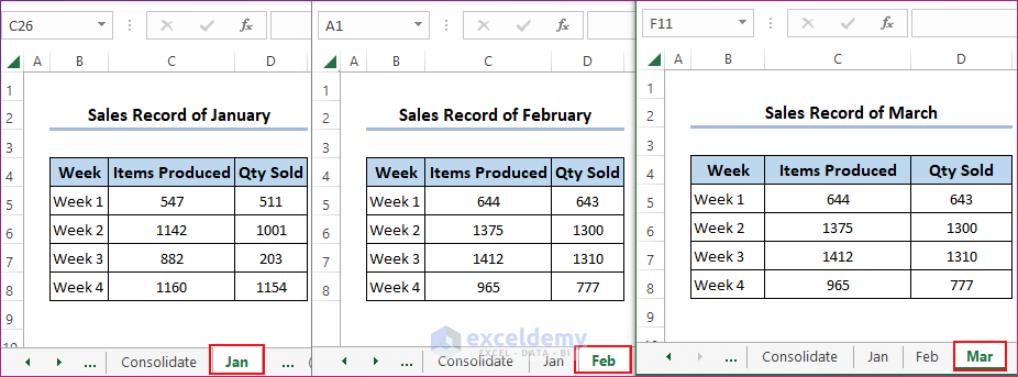
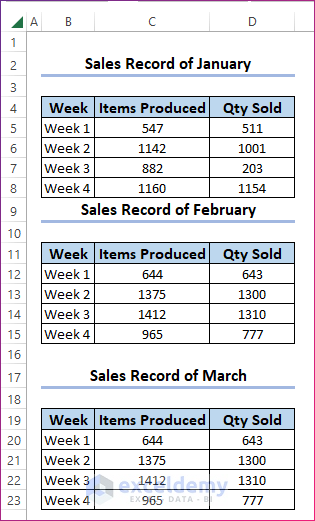
We have a new workbook with three worksheets, each having a sales record of four weeks in January, February, and March, respectively. We’ll collect data from these three worksheets and arrange them in one worksheet.

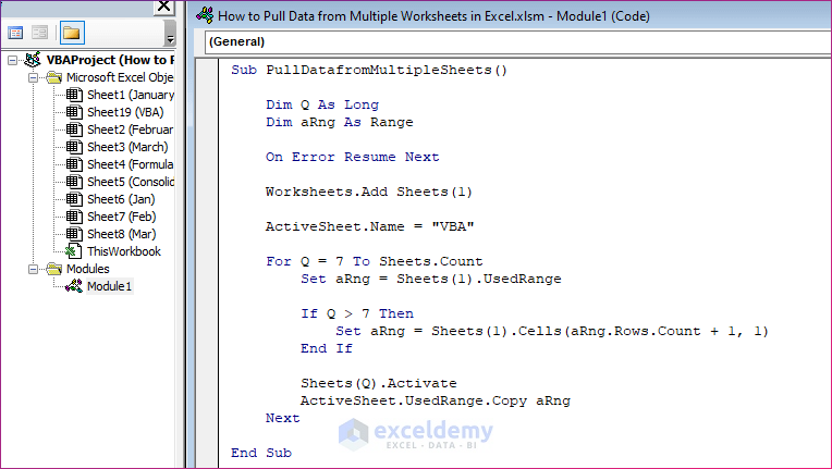
VBA CODE:

Sub PullDatafromMultipleSheets()

    Dim Q As Long
    Dim aRng As Range

    On Error Resume Next

    Worksheets.Add Sheets(1)

    ActiveSheet.Name = "VBA"

    For Q = 7 To Sheets.Count
        Set aRng = Sheets(1).UsedRange

        If Q > 7 Then
            Set aRng = Sheets(1).Cells(aRng.Rows.Count + 1, 1)
        End If

        Sheets(Q).Activate
        ActiveSheet.UsedRange.Copy aRng
    Next

End Sub

Steps:

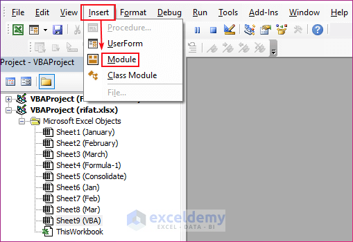
• Press Alt+F11 and go to the VBA editor.
• Go to the Insert tab and click on Module. A new module will be opened.

• Copy the code from above and paste it here.

• Save the Excel file by pressing Ctrl + S.
• You’ll get a notification window.

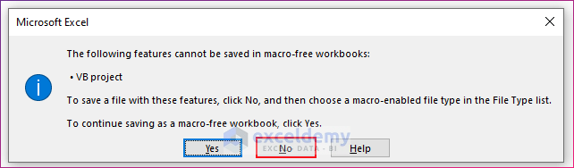
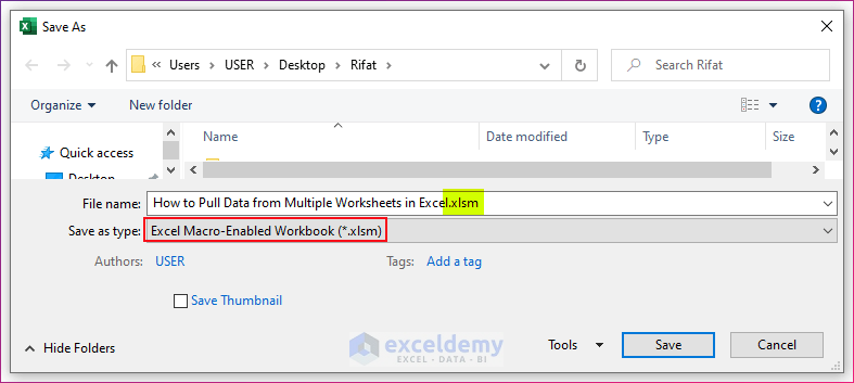
• Click on No and save the file as a Macro-Enabled file (.xlsm).

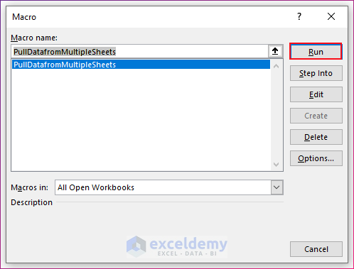
• Click on the Run button or press F5 or press Alt + F8.
• A dialog box called Macro will appear. Select the Macro PullDatafromMultipleSheets and click on Run.

• You will find the data from the three worksheets arranged vertically in a new worksheet called VBA.

Read More: Extract Data from One Sheet to Another Using VBA in Excel

Method 4 – Using Power Query to Pull Data from Multiple Worksheets

Power Query is available from Excel 2016. If you use any older version, you have to download and install it manually.

Steps:

• Go to the first sheet.
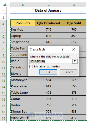
• Select any cell inside the data and press Ctrl + T.
• Confirm that the range contains the entire dataset and check the box in the dialog.
• Press OK.

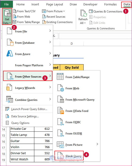
• Go to Data and select Get Data under the Get & Transform Data section from any worksheet.
• Click on the drop-down menu.
• Choose From Other Sources and select Blank Query.

• The Power Query Editor will open.
• In the Formula bar, use this formula:

Power Query is case-sensitive.

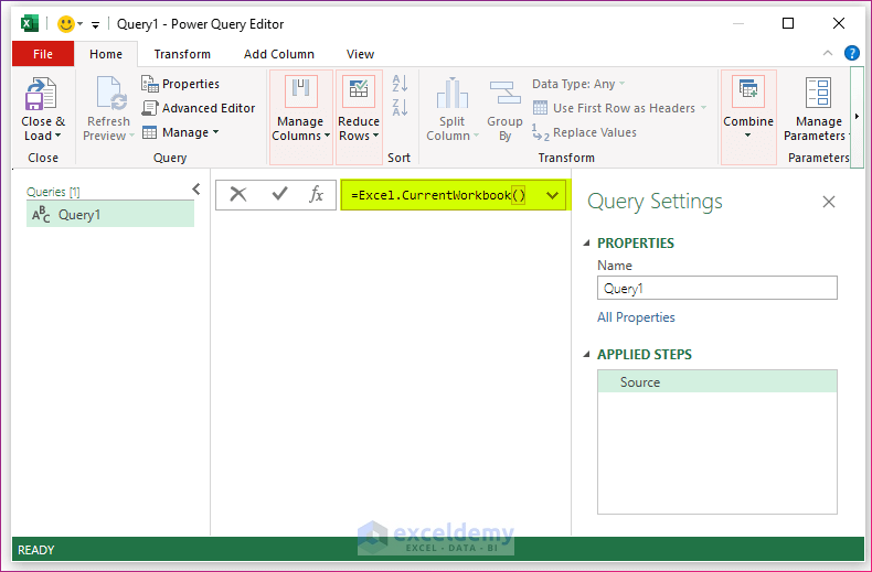
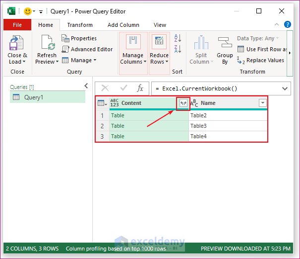
• Click on Enter.
• You will find the three tables from the three worksheets arranged one by one.
• Select the ones that you want to pull. For this example, select all three.
• Click the small right arrow beside the title Content.

• You will get a small box. Click on Expand and then check (put a tick on) all the boxes.

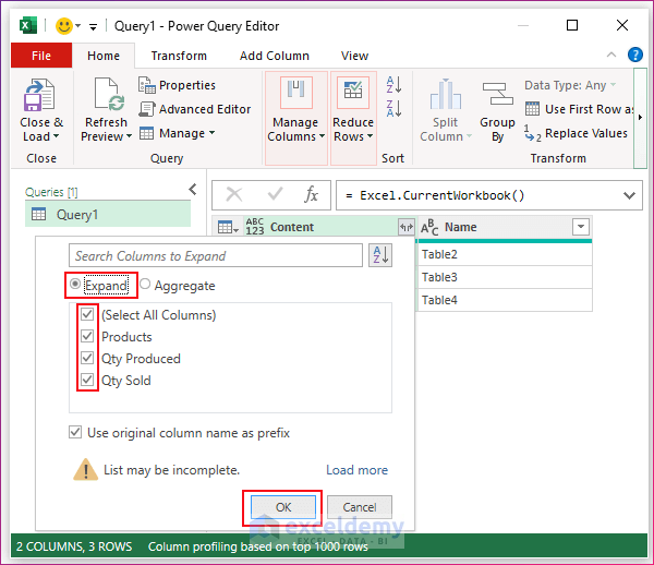
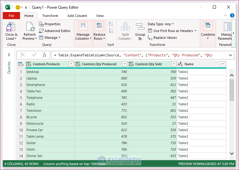
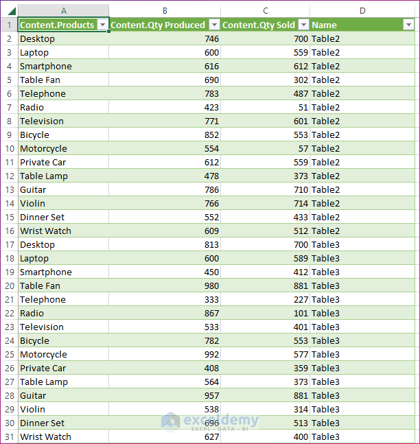
• Click OK. You will find all the items from three tables brought to a single table in Power Query Editor.

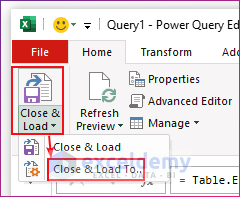
• Go to File and select the Close and Load To… option in the Power Query Editor.

• You will get the Import Data dialog box. Choose Table.
• If you want the combined table to be in a new worksheet, choose New Worksheet. Otherwise, choose Existing Worksheet and enter the cell reference of the range where you want the table.

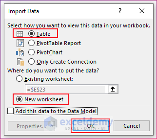
• Click OK. You will find the data from the three worksheets arranged in a single table in a new worksheet named Query.

Read More: How to Pull Data From Another Sheet Based on Criteria in Excel

Download the Practice Workbook

Related Articles

• Extract Filtered Data in Excel to Another Sheet
• How to Pull Values from Another Worksheet in Excel
• Pull Same Cell from Multiple Sheets into Master Column in Excel
• Excel Macro: Extract Data from Multiple Excel Files
• How to Get Data from Another Sheet Based on Cell Value in Excel

<< Go Back To Extract Data Excel | Learn Excel