Doing repetitive work is exhausting sometimes in Excel. We are going to show Excel workflow automation to make your work better. Repetitive work can be done by creating Macros with VBA code in Excel. There are some examples of repetitive work are given below:
- Doing the same type of calculation on all sheets
- Creating and Renaming sheets
- Refreshing Pivot Table when main table data has changed

Excel Workflow Automation: 4 Effective Examples
In this article, we are going to show some Excel workflow automation processes so that you can apply them to ease your work. If you can understand this article you can easily have a better view of this topic and we are providing better suggestions for automating boring work to make your life better.
1. Automating Profit Calculation Using VBA
In this example we are going to automate Profit Calculation using VBA code in every single sheet you will add in your work space easily. We are using Number of Sales of different -product of mobile, Price per mobile and Cost per Mobile to calculate total profit and automate the calculation through all sheets.
Steps:
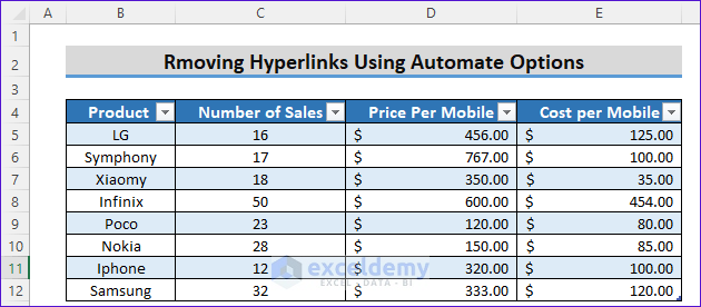
- Here, we are going to use the dataset of Sales of Mobile of different companies.

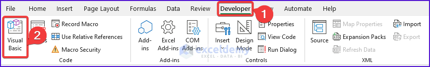
- Later, we will go to Developer >> Visual Basic.

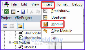
- Subsequently, we will go to Insert >> Module . Then we insert VBA codes in the new Module.

- Thereafter, a VBA Module for the sheet will appear. We are going to use the VBA code given below to find out Total Sales, Total Cost and Profit. You can calculate these parameters in all sheets if you use the similar data table in those sheets.
Sub RunThroughAllSheet()
    Dim jm_ws As Worksheet
    Application.ScreenUpdating = False
    For Each jm_ws In Worksheets
        jm_ws.Select
        Call ProfitCalculation
    Next
    Application.ScreenUpdating = True
End Sub
Sub ProfitCalculation()
    Range("G5") = "=SUMPRODUCT(C:C,D:D)"
    Range("H5") = "=SUMPRODUCT(C:C,E:E)"
    Range("I5") = "=G5-H5"
End Sub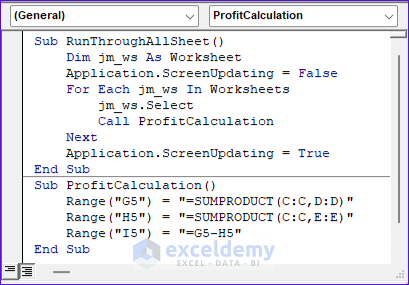
Code Explanation:
- First, we have created a RunThroughAllSheet subroutine to go through all sheets to find the data chart and if it is found it will call the ProfitCalculation subroutine.
- In the ProfitCalculation subroutine, we set some formulas in the cells G5, H5, and I5. The SUMPRODUCT formula in G5 and H5 will return the Total Sales and Total Cost respectively. The formula in I5 will show us the overall Profit. We used the VBA Range property to set the formulas in the corresponding cells.
- Now we will create a button to automate the profit calculation. For that purpose, we select Developer >> Insert >> Button (Form Controls)

- Then, the Assign Macro dialog box will appear.
- After that, we will choose the Macro named RunThroughAllSheet.
- Later, click OK.
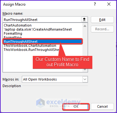
- Then, we will get an option embedding that Macro, and we are going to rename it as Profit Calculation.
- Click on the button and you will see the Total Sales, Total Cost, and Profit.
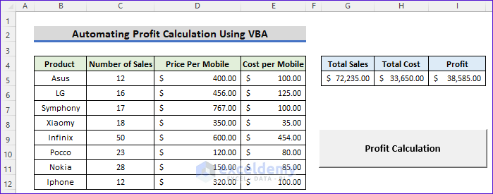
- Consequently, if you change any of the data, Total Sales, Total Cost, and Profit will change.

Now every time you click on the option it will calculate profit for you in every available sheet.
2. Automating Refresh Pivot Table and Charts
In this section, we are going to Refresh a PivotChart automatically. You do not have to Right-click and refresh anymore to update the PivotChart if you change any data. Let’s have a look at the description below to get a better idea of this type of workflow automation.
- First, we are going to create a Data Table like below.

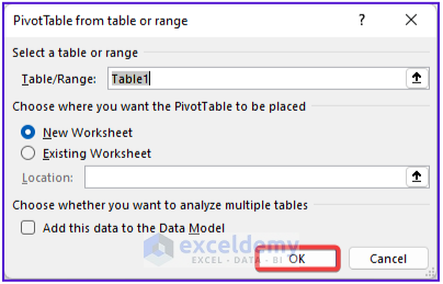
- Then, we will go to Insert >> PivotTable and select from Table Range.
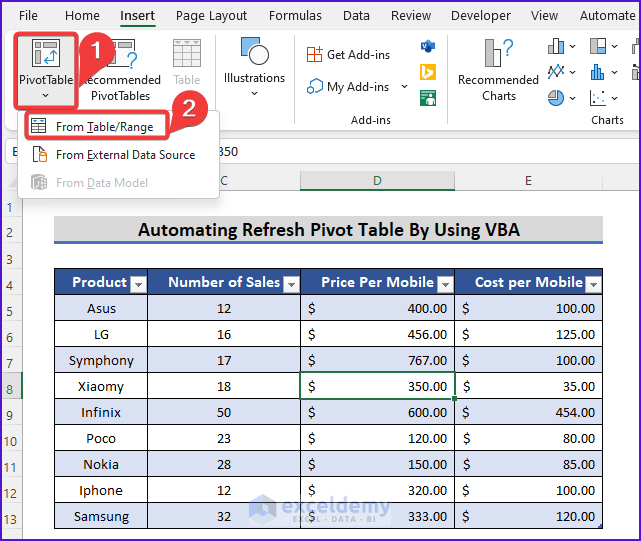
- After that, we are going to use the whole table and select OK.
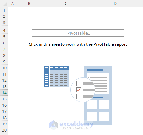
- Then we will get a blank PivotTable.
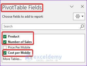
- After that, you can see the PivotTable Fields on the right side of the Excel sheet. Check Product, Number of Sales, and Cost per Mobile.
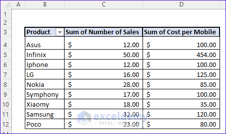
- Now, you will get the Pivot Table.
- Then, we will select PivotTable Analyze >> PivotChart.
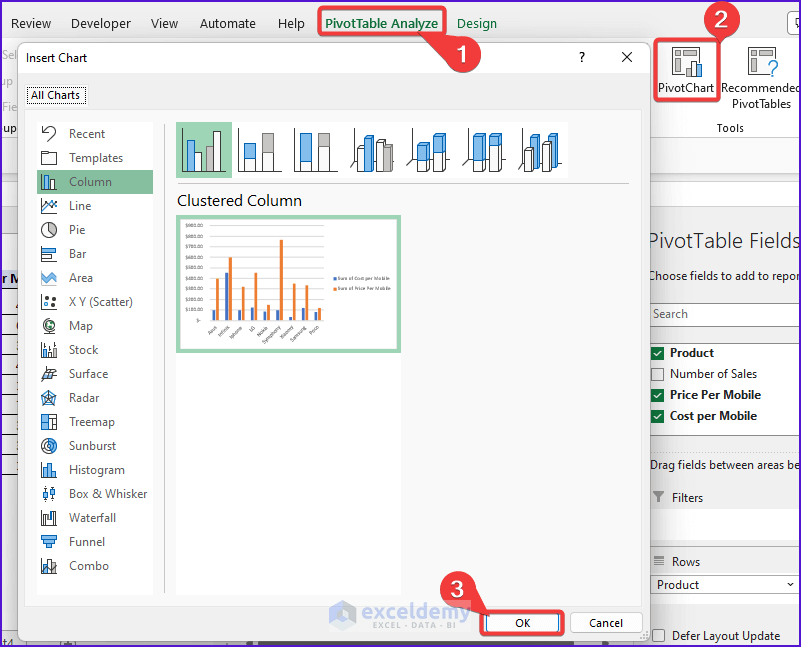
- After that, you will get the graph automatically.

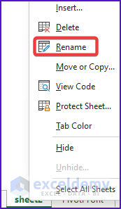
- Now, we are going to rename the new sheet.
- Then, we will go to View Code.

- After that, we are going to upload the code below.
Private Sub Worksheet_Change(ByVal jm_Target As Range)
Worksheets("PivotChart").PivotTables("PivotTable1").PivotCache.Refresh
End Sub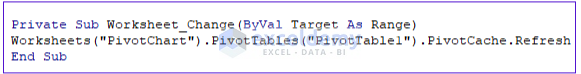
- This will refresh the PivotTable instantly if any changes are made in the mother chart.
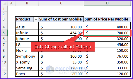
- Let’s make a change in the data of the mother table.
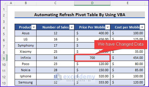
- Now, data from Pivot Datatable will change without Refresh.
- After that, the graph will automatically change without Refresh.
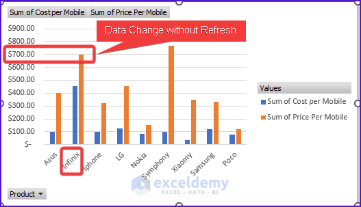
After that, you will not need to refresh data. It will always refresh itself.
Thus you can automate the workflow of a PivotChart.
3. Creating and Renaming Worksheets Automatically
In this article we are going to create a custom name when you create a new sheet, It will easily rename every sheet as soon as you give the custom Shortcut Key.
Steps:
- Later, we will go to Developer >> Visual Basic.
- Subsequently, we will go to Insert >> Module. Then we insert VBA codes in the new Module.
- Then, you upload the following code. This code will create a new sheet and rename the sheet as Sales1 and Sales2, not Sheet1 and sheet2.
Sub CreateAndRenameSheet()
    If ThisWorkbook.Sheets.Count < 255 Then
        Dim newSheet As Worksheet
        Set newSheet = ThisWorkbook.Sheets.Add
        newSheet.Name = "Sales" & ThisWorkbook.Sheets.Count
    Else
        MsgBox "The number of sheets in the workbook has reached the limit."
    End If
End Sub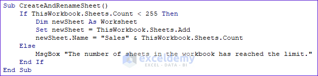
Code Explanation:
- Here, we have created a variable newSheet for Worksheet
- Then, we added a new sheet by ThisWorkbook.Sheets.Add. This method will dynamically create a new worksheet in your workbook.
- Subsequently, newSheet.Name will dynamically rename your sheet as you want.
- You can change the name from newSheet.Name = “Sales” & ThisWorkbook.Sheets.Count.
- Then we are going to create a Shortcut Key as ctrl + p. Every time you use ctrl+p it will automatically create a new sheet naming Sales1, Sales2, Sales3, and so on.

It will automatically rename files according to what you want.
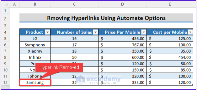
4. Removing Hyperlink Using Excel Automate Option
In this section, we are going to create an arbitrary dataset and embed hyperlinks and after that, we are going to remove Hyperlinks using Automate >> Remove Hyperlinks from Sheet.
Steps:
- First, we are going to create an arbitrary data table like below.
- Then we will embed Hyperlinks in data.
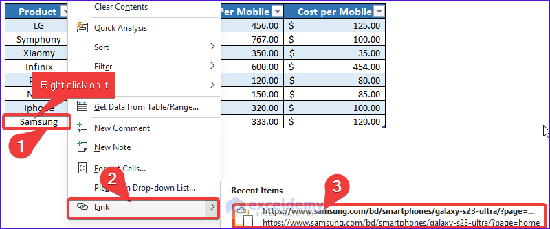
- After that, we are going to press Insert Link.. and add it to your file name.

- Then we finally get the Hyperlinked data.

- Now we are going to Automate >> Remove Hyperlinks from Sheets then get rid of the Hyperlinks.

- Then, we will Select Run from Code Editor.
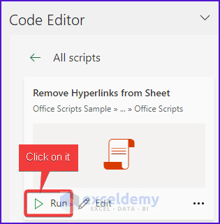
- Then finally we will get the hyperlink removed.
Download Practice Workbook
You can download the practice workbook from the following download button.
Conclusion
In this article, we have given you some ideas and examples of Excel workflow automation. You can automate anything you want using VBA Macro. Please comment below if you have any queries. We will try to solve the isssue.
Related Articles
- How to Create a Workflow in Excel
- How to Create Workflow Chart in Excel
- How to Create Workflow Management Template in Excel
- How to Create Approval Workflow in Excel
- How to Create a Workflow Tracker in Excel
<< Go Back to Workflow in Excel | SmartArt in Excel | Learn Excel
Get FREE Advanced Excel Exercises with Solutions!
