Microsoft Excel is one of the most useful software you can get. Using Excel’s features and tools, it is possible to do an infinite number of things with a dataset. We need to use Excel charts to show the workflow graphs for many companies regularly. Workflow diagrams are one of the best ways to show how business systems work. In this article, we’ll look at two easy ways to show how workflow charts work in Excel. Therefore, review these two suitable ways to create a Workflow Chart in Excel.
Workflow Chart in Excel: 2 Suitable Ways to Create
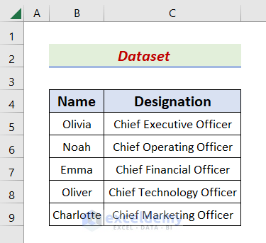
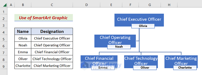
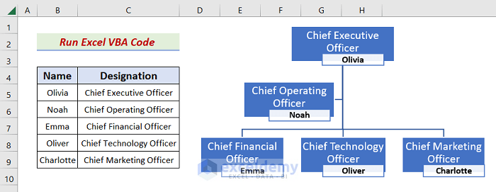
To illustrate this point, let’s examine a representative dataset. Name and Designation are columns in the following dataset. Using the dataset’s information, we will create a workflow diagram. This article’s first method explains how to represent workflow diagrams using the SmartArt feature. In comparison, another generates a workflow-illustrating graph in Excel using Visual Basic for Applications (VBA). In addition, I’ve been using Microsoft Excel 365 to compose this post. You are free to select the version that best meets your needs. Whichever option you choose is acceptable to us.
1. Utilize SmartArt Graphic to Generate Workflow Chart in Excel
With SmartArt Graphic, you can make and modify professional-looking diagrams instead of just using plain text to describe processes. Smart Art facilitates the development of structures, frameworks, and procedures. As part of this talk, we’ll build a workflow diagram using SmartArt. Please read these instructions thoroughly and attentively and follow them to the completion of the job.
STEPS:
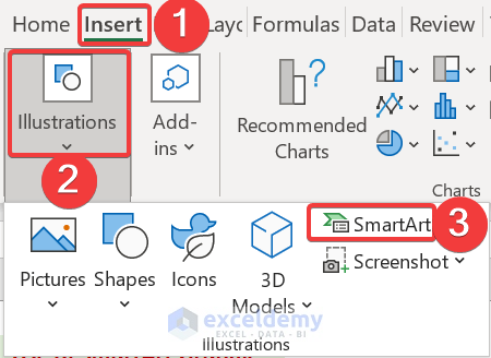
- First of all, from your Insert tab, go to,
Insert → Illustrations → SmartArt
- Subsequently, the SmartArt Graphic window will appear.
- After that, pick the Hierarchy option on the left side and select the Name and Title Organization Chart.
- Later, hit the OK button.

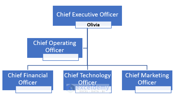
- Consequently, an empty workflow diagram will open like the one below.

- At this point, click the Title Box on the top and go to the Home tab.
- Next, make the Font size 14 and click the B icon.

- Now, type the value of C5, then click anywhere in the workflow graph.
- Thus, it will produce the intended outcome as follows.

- Sequentially, we need to do the same procedure for the rest of the Title Boxes and input the value of the Column C.
- At this stage, we will find the workflow chart below.

- Presently, click in the Name Box and go to the Home tab.
- Later, from the Alignment group, select the Middle and Center align.
- Next, from the Font group, choose the B symbol to bold the text.

- Then, input the value of B5 in the Name Box.
- At this time, click anywhere in the workflow graph area to see the below outcome.
- Likewise, follow the same procedure for the other Name Boxes and type the values with the B symbol.
- Finally, click anywhere in the sheet to display the workflow chart.
2. Run an Excel VBA Code to Create Workflow Chart
Visual Basic for Application is shortened as VBA. Microsoft created VBA. We can access Excel-incompatible functions via VBA code. VBA in Excel is another exciting way to visualize chart problems. We’ll graph a workflow chart in Excel using VBA in this lesson. You can also perform workflow automation in Excel. Please follow these directions to finish the assignment.
STEPS:
- To begin, choose the desired sheet as the Active sheet.
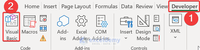
- Second, go to the Developer tab.
- Third, click the Visual Basic icon.
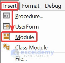
- After that, select Insert followed by Module.
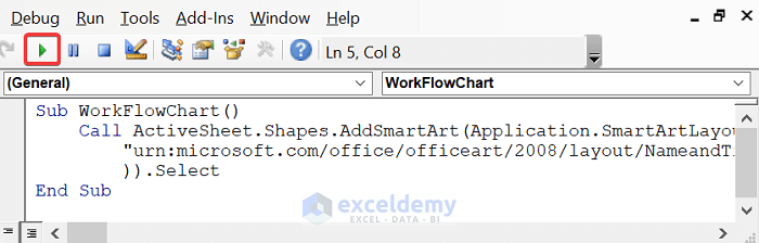
- Now, type the following code in the Module Box.
Sub WorkFlowChart()
    Call ActiveSheet.Shapes.AddSmartArt(Application.SmartArtLayouts( _
        "urn:microsoft.com/office/officeart/2008/layout/NameandTitleOrganizationalChart" _
        )).Select
End Sub- Later, press F5 or tap the Run button.
- As a consequence of this, an empty workflow graph will appear like the one below.

- Next, click the Title Box at the top and navigate to the Home tab.
- Then, adjust the Font size to 14 and click the B icon.

- Later, enter C5‘s value and click anywhere on the workflow diagram.
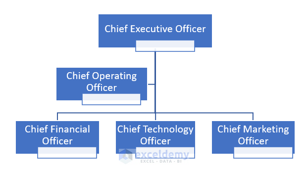
- Consequently, the expected result will be as follows:

- Presently, we must repeat this process for the remainder of the Title Box and enter the value of Column C.
- At this point, the workflow diagram is shown below.
- Currently, click the Name Box and go to the Home tab.
- Later, select the Middle and Center alignment from the Alignment group.
- Next, select the B symbol from the Font category to bold the text.

- Then, enter B5‘s value in the Name Box.
- Afterward, click anywhere within the workflow graph region to view the result.

- Similarly, repeat the same approach for the second Name Box and enter the column B.
- Click anywhere on the sheet to reveal the workflow diagram.
Download Practice Workbook
Please click on the link below this paragraph if you want a free copy of the example workbook we referenced during the presentation.
Conclusion
Following the procedures we covered, you will soon be able to create a Workflow Chart in Excel. Keep utilizing them, and please share any more suggestions or better methods. Remember to share your thoughts, questions, and recommendations in the space provided.
Related Articles
- How to Create Workflow Management Template in Excel
- How to Create Approval Workflow in Excel
- How to Create a Workflow Tracker in Excel
<< Go Back to Workflow in Excel | SmartArt in Excel | Learn Excel
Get FREE Advanced Excel Exercises with Solutions!
