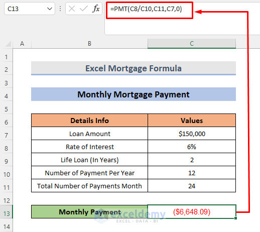
Example 1- Formula to calculate the Monthly Mortgage Payment in Excel
Consider that you want to start a business and take a loan: $150,000 (C7).
The annual interest rate is 6% (C8), the duration is 2 years (C9) and the loan is paid monthly.
STEPS:
- Select a cell to calculate the monthly payment. Here, C13.
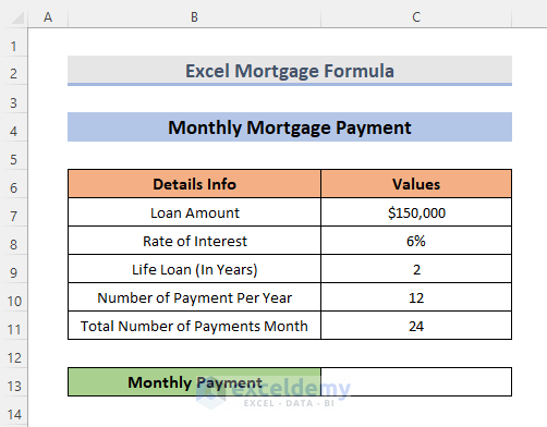
- Enter the formula.
=PMT(C8/C10,C11,C7,0)- Press Enter.
- The monthly mortgage payment is displayed.
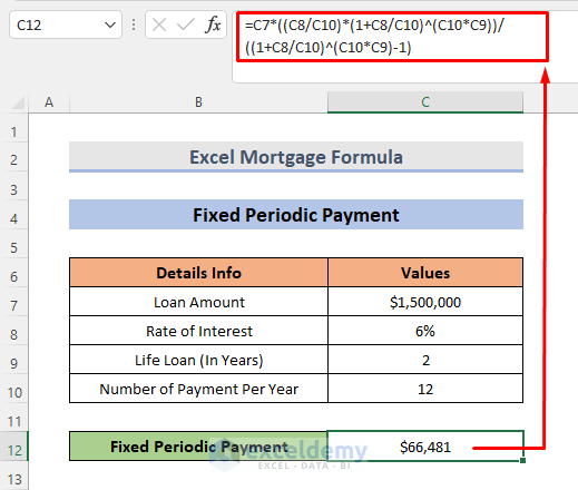
2. Excel Mortgage Formula to calculate the Fixed Periodic Payment
The loan amount is $150,000 (C7).
The annual interest rate is 6% (C8), the duration is 2 years (C9) and the total number of months is 12 (C10).
STEPS:
- Select a cell to calculate the monthly payment. Here, C12.
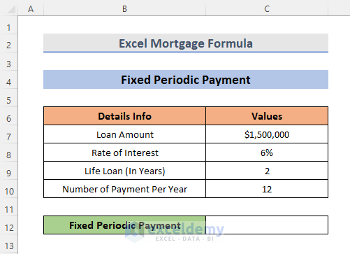
- The generic formula for a fixed periodic payment is:
=loan amount((rate of interest/number of payment per year)*(1+rate of interest/number of payment per year)^(number of payment per year*life loan))/((1+rate of interest/number of payment per year)^(number of payment per year*life loan)-1)- Enter the formula.
=C7*((C8/C10)*(1+C8/C10)^(C10*C9))/((1+C8/C10)^(C10*C9)-1)- Press Enter.
The fixed periodic payment is displayed.
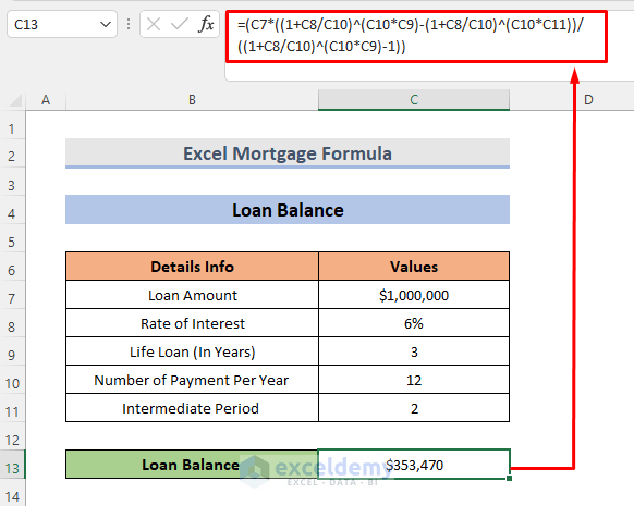
3. Find the Outstanding Loan Balance
To find the outstanding loan balance, slight modifications were made to the dataset: the loan amount was decreased and the duration of the loan increased.
Calculate the outstanding loan amount with one intermediate period.
STEPS:
- Select a cell to see the result. Here, C13.
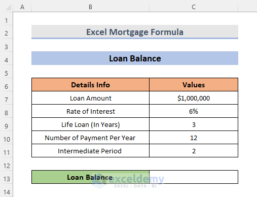
- The generic formula for a fixed periodic payment is:
=loan amount((rate of interest/number of payment per year)*(1+rate of interest/number of payment per year)^(number of payment per year*life loan))-((1+rate of interest/number of payment per year)^(number of payment per year*life loan)-1))- Enter the formula.
=(C7*((1+C8/C10)^(C10*C9)-(1+C8/C10)^(C10*C11))/((1+C8/C10)^(C10*C9)-1))- Press Enter.
The result is displayed in C13.
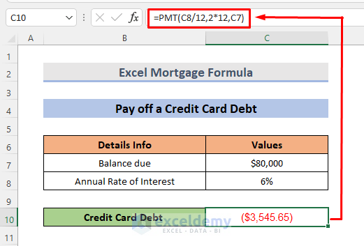
Example 4 – Using a Mortgage Formula to Calculate the Monthly Payments for a Credit Card Debt
Consider the due balance and the annual interest rate in C7 and C8.
STEPS:
- Select C10.
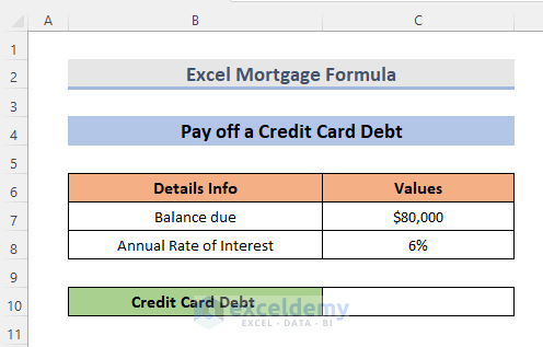
- Enter the following formula:
=PMT(C8/12,2*12,C7)- Press Enter.
This is the output.
Example 5 – Using an Excel Mortgage Formula to calculate the Principal Amount Repayment in the 24th Month
STEPS:
- Calculate the loan balance in period 1. Select C14.
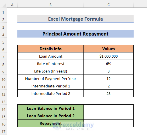
- The generic formula for a fixed periodic payment is:
=loan amount((1+rate of interest/number of payment per year)^(number of payment per year*life loan))-((1+rate of interest/number of payment per year)^(number of payment per year*intermediate period 2))/(((1+rate of interest/number of payment per year)^(number of payment per year*life loan)-1)- Enter the formula:
=(C7*((1+C8/C10)^(C10*C9)-(1+C8/C10)^(C10*C11))/((1+C8/C10)^(C10*C9)-1))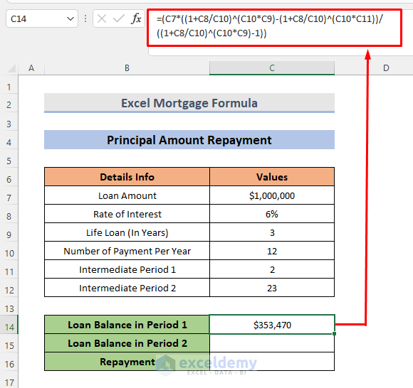
- Press Enter.
- The generic formula for a fixed periodic payment is:
=loan amount((1+rate of interest/number of payment per year)^(number of payment per year*life loan))-((1+rate of interest/number of payment per year)^(intermediate period 2))/((1+rate of interest/number of payment per year)^(number of payment per year*life loan)-1)- For the loan balance in period 2, the formula is:
=(C7*((1+C8/C10)^(C10*C9)-(1+C8/C10)^(C12))/((1+C8/C10)^(C10*C9)-1))- Press Enter.
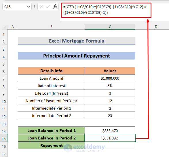
- Subtract the loan balance in period 1 from the loan balance in period 2. The formula will be:
=C15-C14
- Press Enter.
You will see the result.
Download Practice Workbook
Download the workbook and practice.
Excel Mortgage Formula: Knowledge Hub
- How to Use Formula for 30 Year Fixed Mortgage in Excel?
- How to Use Formula for Mortgage Principal and Interest in Excel?
- How to Use Formula for Car Loan Amortization in Excel?
<< Go Back to Excel Formulas for Finance | Excel for Finance | Learn Excel
Get FREE Advanced Excel Exercises with Solutions!
