Sometimes you may need to use an implicit intersection operator in Excel. In this article, I will show you how, and where to use an implicit intersection (@) operator in Excel.
However, if you are a user of the Microsoft 365 version of Excel, then most of the time you mayn’t need to use the @ operator. Now, let’s know the details about this @ operator.
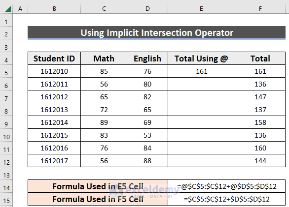
Below, I have attached a screenshot as an overview of the article, representing the applications of the implicit intersection operator in Excel. You’ll learn more about the usage of the @ operator properly in the following sections of this article.
What Is an Implicit Intersection Operator?
Suppose you have a range of data. Now, if you use the implicit intersection operator (@) in any formula for that entire range still it will give the value for a particular single cell. So, the @ operator decreases the output of a range into one single output for a cell.
Implicit Intersection Operator in Excel: 4 Examples
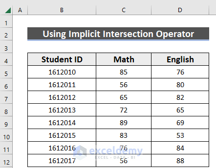
Here, I will demonstrate 4 suitable and simple examples with detailed steps on how to use the implicit intersection operator in Excel. For your better understanding, I am going to use the following dataset. Which contains three columns. Those are Student ID, Math, and English. The dataset is given below.
1. Applying Implicit Intersection Operator in Functions
Here, I will show you the application of the @ operator in functions. Actually, there are some functions where you must use the implicit intersection operator, even in the Excel 365 version. Moreover, if you don’t use the @ operator then you will get a warning for using it.
On the other hand, some functions don’t support the implicit intersection operator.
1.1 Use of VLOOKUP Function with Implicit Intersection Operator
Now, I will show you the utilization of the VLOOKUP function in the case of an implicit intersection operator. When you use an entire column in this VLOOKUP function then there is a chance to be of Spill Error. Thus, you should use the @ operator which will reduce the output for a single cell.
Now, for your understanding see the following example.
Suppose you want to find out the marks of English for each student in a new column named English (column G).
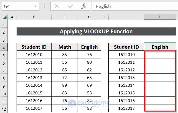
Steps:
- First, write the following formula in the G5 cell.
=VLOOKUP(F:F,B:D,3,0)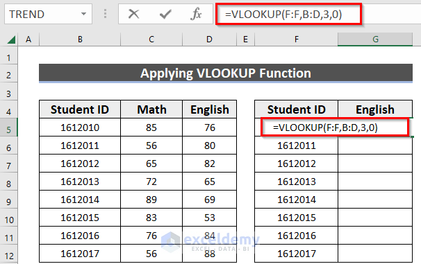
🔎 Formula Breakdown:
- Here, F:F (entire F column) is the lookup_value.
- Then, B:D is the table_array from where the VLOOKUP function will search for values.
- 3 is the Column_Index number. Which means it will return the marks from the English column.
- 0 denotes the exact_match.
- Then, press ENTER.
After pressing ENTER, you will get a notice from Microsoft Excel where the Excel will suggest you use the implicit intersection operator.
- Then, press the Yes button to accept Microsoft Excel’s suggestion.
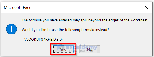
As a result, you see the English mark of Student ID 1612010. So, the modified formula is:
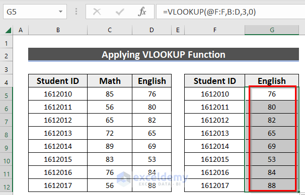
=VLOOKUP(@F:F,B:D,3,0)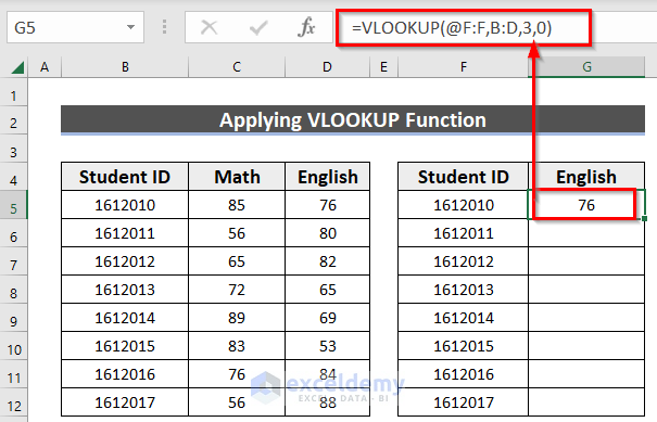
- Now, drag the Fill Handle icon to paste the used formula to the other cells of the column and you will get the marks for all students.
Read More: Intersection of Row and Column in Excel is Called a Cell
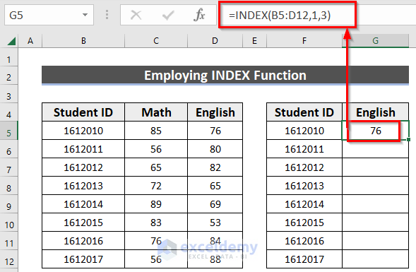
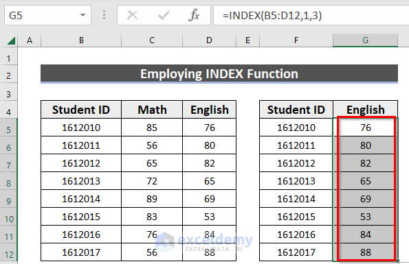
1.2 Implicit Intersection Operator with INDEX Function
Now, for the previous example, I will use the INDEX function with the implicit intersection operator, and let’s see what happens.
Steps:
- First, write the following formula in the G5 cell.
=@INDEX(B5:D12,1,3)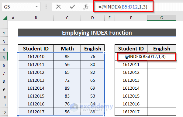
🔎 Formula Breakdown:
- Here, B5:D12 is the reference_array from where the INDEX function will return values.
- Then, 1 is the row_number. Which means it will return the value from the 1st row of the given array.
- 3 is the column_number. Which means it will return the value from the English column.
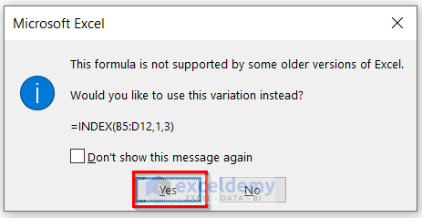
- After pressing ENTER, you will see the following suggestion from Microsoft Excel where the Excel will suggest you remove the implicit intersection operator.
- Then, press the Yes button to accept Microsoft Excel’s suggestion.
Lastly, you will get marks in English for ID 1612010.
- Then, drag the Fill Handle icon to paste the used formula to the other cells of the column and you will get the marks for all students.
Read More: Intersection of Two Columns in Excel
2. Using Implicit Intersection Operator in Generic Formula
Here, I will show you a simple generic formula and the behavior of the implicit intersection operator.
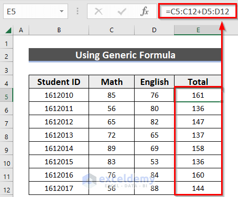
Suppose you want to find out the total marks for all the students.
- So, I will use the simple formula in the E5 cell.
=C5:C12+D5:D12- Subsequently, press ENTER, and you will get the total marks for all the students in one click.
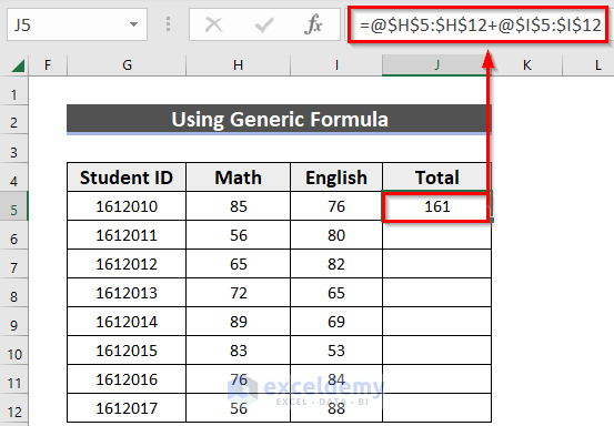
- Now, let’s use the implicit intersection operator in the J5 cell.
=@$H$5:$H$12+@$I$5:$I$12- Then, press ENTER, and you will get the total marks of only one student.
Here, in this formula, I have added two ranges but still, it returns a single output using an @ operator. Additionally, the dollar sign ($) will fix the cell’s position.
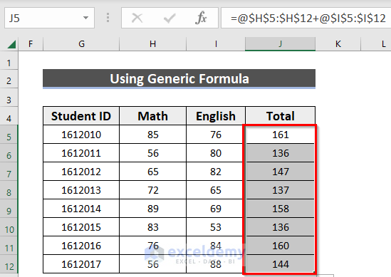
- After that, drag the Fill Handle icon to paste the used formula respectively to the other cells of the column and you will see all the student’s total marks.
3. Employing Implicit Intersection Operator in Table
The most important use of implicit intersection operator is, in Excel Table. Basically, with the help of this @ sign, you can call not only any column of the table but also the entire table.
Now, let’s have the following Excel table named Table_Marks, which has those three columns Student ID, Math, and English.
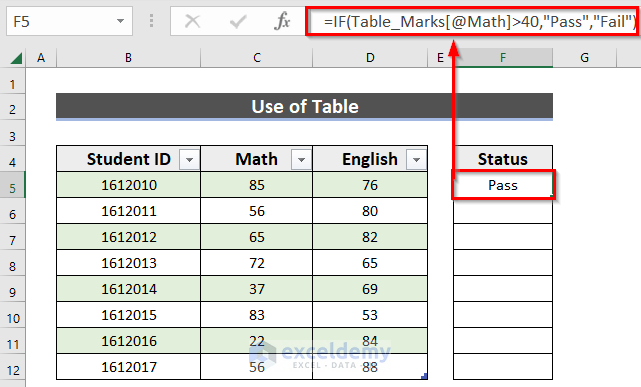
At this moment, I want to know the remarks based on the Math marks of every student in the Status column.

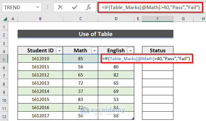
- So, I will use the IF function to find out the status based on marks in Math. Here, after writing “=IF(@ta” you will get some options including the Table_Marks.
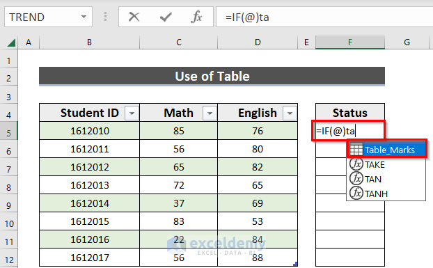
- Now, write the corresponding formula in the F5 cell.
=IF(Table_Marks[@Math]>40,"Pass","Fail")Here, you can’t use the @ sign twice to call the table and the particular column.
- Consequently, press ENTER to get the status.
🔎 Formula Breakdown:
- Firstly, the IF function will return an output of a given logical test. Which is whether the marks in the Math column are greater than 40 or not. Here, Table_Marks[@Math] is mentioned as the column of Math of Table_Marks. 3rd bracket secures the name of the column header.
- Secondly, “Pass” —> When the logical test is TRUE then it will return Pass. Basically, an Inverted Comma is a must for getting a text as the output.
- Thirdly, “Fail” —> denotes that when the logic fails then it will return Fail.
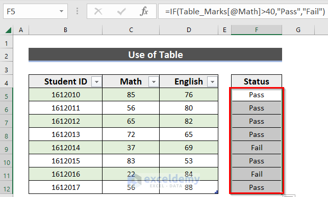
- After that, drag the Fill Handle icon to paste the used formula to the other cells of the column and you will get the status for all students.
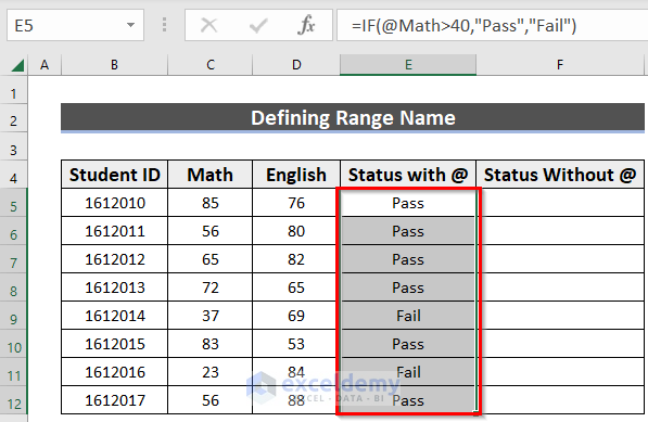
4. Use of Implicit Intersection Operator for Calling a Range
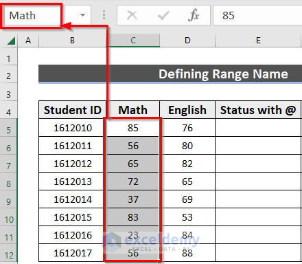
Another important use of the implicit intersection operator is for mentioning a range. To do so, I need to give a name of that certain range. Now, let’s see the steps below.
Steps:
- First, select all the data of a column and then write a name in the Functions box.
- Then, press ENTER. Here, I have named the data having marks of math as Math.
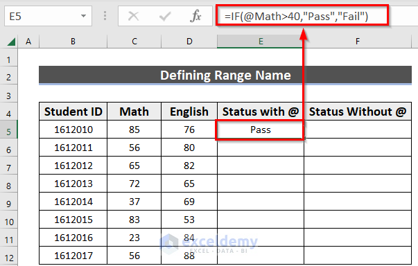
- Then, you can mention the whole range for your formula like the following one.
=IF(@Math>40,"Pass","Fail")- Subsequently, press ENTER.
Here, for the use of an @ operator, you will get a single output, like only the status for the particular ID 1612010.
🔎 Formula Breakdown:
- Firstly, the IF function will return an output of the given logical test. Which is whether the marks of the data range named Math are greater than 40 or not. Here, @ is used to call the data range.
- Secondly, “Pass” —> When the logical test is TRUE then it will return Pass. Basically, an Inverted Comma is a must for getting a text as the output.
- Thirdly, “Fail” —> denotes that when the logic fails then it will return Fail.
- After dragging the Fill Handle icon, you will get all the statuses.
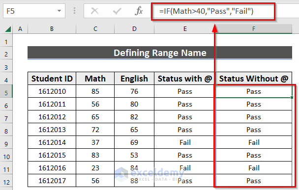
- On the other hand, if you don’t use the @ operator here, then you will find all the statuses at one press of the ENTER button.
Read More: Performing Intersection of Two Data Sets in Excel
How to Use Intersect Operator in Excel
There is another operator in Excel, named intersect operator. Actually, this is a single space that works as an intersect operator. Now, for the below screenshot. Where I have chosen the C column then keep a space and choose the 5th row. As a result, it will return the value, where the column intersects the row.
- So, the formula becomes:
=C4:C12 B5:D5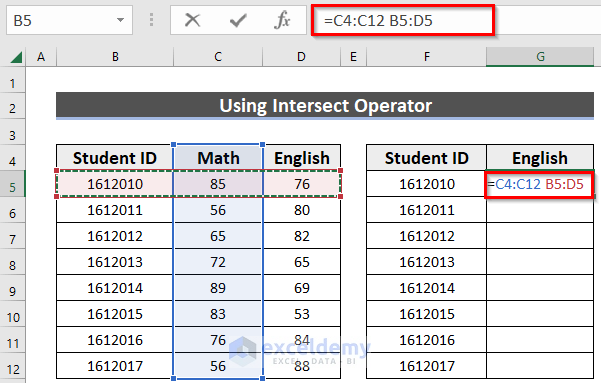
- After pressing ENTER, you will get the following value.

Read More: How to Use Intersection Operator in Excel
Practice Section
Now, you can practice the explained methods by yourself.
Download Practice Workbook
You can download the practice workbook from here:
Conclusion
I hope you found this article helpful. Here, I have described how to use the implicit intersection operator in Excel. Please drop comments, suggestions, or queries if you have any in the comment section below.
<< Go Back to Excel Intersection | Excel Operators | Excel Formulas | Learn Excel
Get FREE Advanced Excel Exercises with Solutions!
