The intersection of row and column is usually called a cell in Excel. Thousands of cell integration creates a whole spreadsheet of Excel. This tutorial will provide a complete overview of rows and columns, properties of cells, cell reference, and cell navigation with proper illustrations.
Basics of Row-Column and Cell in Excel
Row and Column
Rows and Columns are two different aspects of Excel that make up a cell.
Rows are the horizontal lines in Excel and are expressed in numbers(1,2,3…). There are 10,48,576 rows in the spreadsheet.
On the other hand, columns are the vertical lines in the spreadsheet and are expressed in alphabets(A, B, C…). The columns range from A to XFD consisting of 16,384 individual columns.
Cell
The intersection of row and column in Excel is usually called a cell. Cells are the rectangle boxes you see in the grid of an Excel spreadsheet.
A cell is the combination of a row and a Column. A cell is attributed to one row and one column. So, cells are expressed in alphanumeric values like A10, D5, etc.
There are precisely 17,179,869,184 cells in a spreadsheet.
Read More: Intersection of Two Columns in Excel
What Is Cell Reference?
Cell Reference is used for conducting a formula in Excel. It refers to a single or a range of cells in a formula (value or property) in order to conduct simultaneous operations in an Excel worksheet. Addressing or referring to a cell follows a definite and structured way. There are two distinguishable cell references.
Relative Reference
Relative references change when a formula is copied to another cell.
For relative cell reference, the cell address looks like this B5, C10, A12.
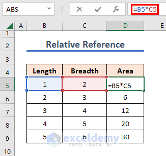
Let’s see an example of a relative reference
We are finding areas of rectangles. For that, we have to multiply Length and Breath.
And as the length and breadth are variable, we have to use relative reference.
The formula used in the area column contains only relative references.
The formula in the D5 cell is:
=B5*C5Both B5 and C5 are taken as relative references.
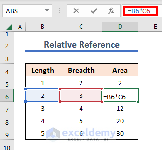
Notice the change in relative reference.
The formula in D6 is:
=B6*C6Where B6 and C6 are also relative references. We didn’t apply an individual formula for each cell. We have just applied the formula in cell D5 and then dragged it down the next cells and the cell references have been changed automatically.
Absolute Reference
Absolute references remain constant no matter where they are copied.
For absolute cell reference, we have to insert the dollar sign ($) in the cell address, for example, $B$5,$C$10,$A$12 etc.
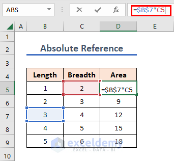
Let’s find out the area using absolute reference.
For that, we will use the same length B7 for all areas.
So the formula in D5 will be:
=$B$7*C5Where $B$7 is the absolute reference.
And, in the D6 cell, the formula is:
=$B$7*C6Where $B$7 is the same absolute reference.

Properties of Cell in Excel
We need to know the basic properties of a cell in an Excel spreadsheet. Let’s discuss these properties.
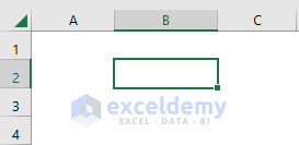
Active Cell
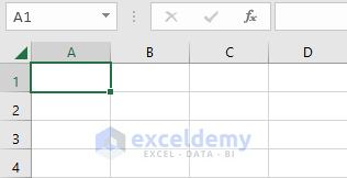
The active cell is the selected cell in which data is entered when you start typing.
Only one cell can be active at a time.
The active cell appears with a green border. In the image below, cell B5 is active.
Cell Address
Every cell has a unique address. When you select a cell the cell address appears on the left side of the worksheet in the Name Box.
Cell Formats
Cell formats allow us only to change the way cell data appears in the spreadsheet.
It only changes how data is presented in a cell and does not alter the data values.
The cell formatting option is used for different data types for Example currency, date, scientific options, time, fractions, etc.
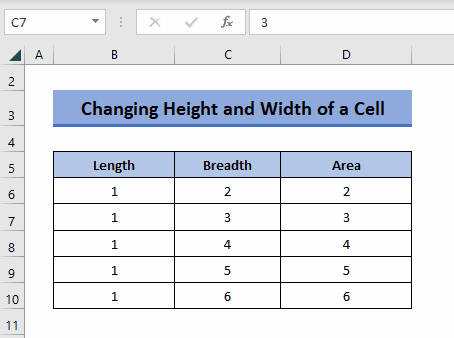
Cell Height and Width
You can change the cell height and width.
The height and width of a cell can be changed manually, using your mouse. Just take your cursor to the edge of the cell, hold and drag your mouse according to your need to change the height and width of the corresponding cell. See the GIF below where we have changed the height and width of cell C7.
Also, you can set cell height and width with the Format option from the Home tab.
Read More: Performing Intersection of Two Data Sets in Excel
Cell Navigation with Keyboard Shortcuts
Let’s see some cell navigation shortcuts.
Accessing Last Cells
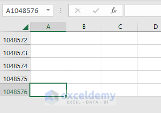
We have set the A1 cell active. In order to navigate quickly to the bottommost cell of this column follow any of these commands: CTRL ⇒ Down Arrow (↓) or End ⇒ Down Arrow (↓)
This command will take you to the bottom cell in column A, which is 1048576th.
Similarly, to access the rightmost cell of a row, you can follow any of these commands:
CTRL ⇒ Right Arrow (→) or END ⇒ Right Arrow (→)
And for the topmost cell,
CTRL ⇒ Up Arrow (↑) or END ⇒ Up Arrow (↑)
Access to Any Cell
To access a random cell press F5.
Write the cell address you want to navigate in the Reference box and press OK.
We inserted F30.
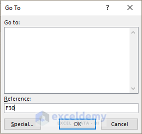
And, this command will take you to the F30 cell.
More Shortcuts
Tab >> This button moves the active cell to the right side.
Shift + Tab >> This command shifts the active cell to the leftmost side.
Home >> This button takes the active cell to the first cell of a row.
Ctrl + Home >> Takes to the first cell of the Excel sheet.
Conclusion
So, now we know the intersection of row and column in Excel is called a cell and this article focuses on different aspects of Excel cells. We hope you will find this article useful. If there are any queries or suggestions, please leave them in the comment section. Have a great day!
Related Articles
<< Go Back to Excel Intersection | Excel Operators | Excel Formulas | Learn Excel
Get FREE Advanced Excel Exercises with Solutions!
