Frequently, you might need to deal with a larger dataset in Excel. What if you want to find the output from the entire dataset that matches your defined partial number instead of the partial string? Certainly, you can accomplish the task using some of the popular Excel formulas along with the wildcard characters. In this instructive session, I’ll show 5 methods to work with partial number match utilizing the formula in Excel with proper explanation.
Formula for Partial Number Match in Excel: 5 Uses
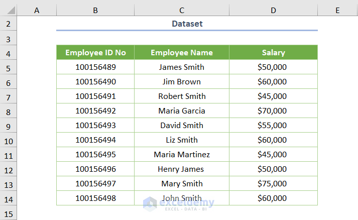
The below screenshot demonstrates today’s dataset where Employee Name is provided with their unique ID No and Salary. Now, you need to perform partial number matching based on the Employee ID No.
Let’s dive into the methods.
1. Using IF and ISNUMBER Functions
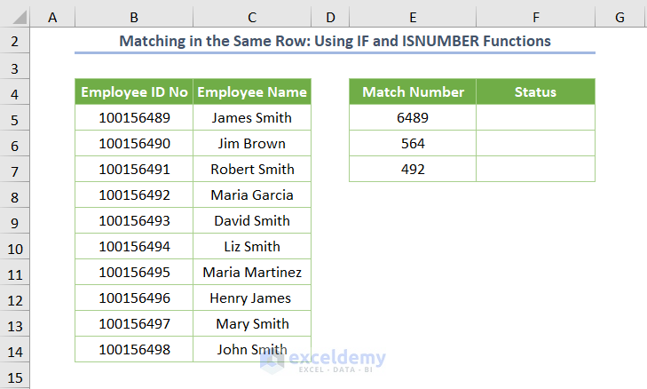
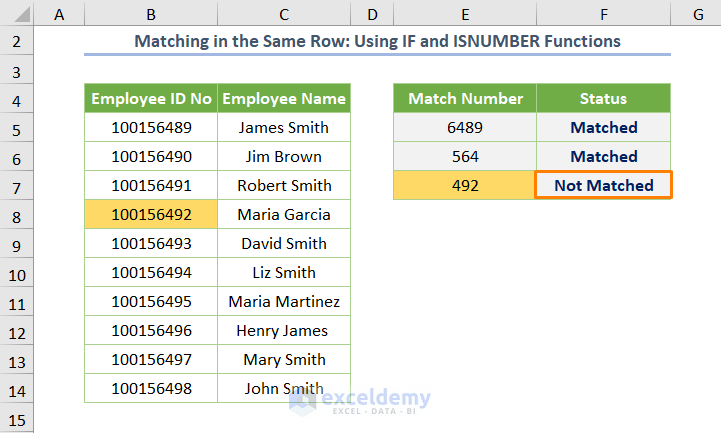
In the beginning method, you’ll see a partial number match in the same row using the IF and ISNUMBER functions. Let me clear this thing.
Assuming that you have the partial match number in the E5 cell and you want to perform the partial number matching based on the B5 cell. That means you want to find the output in the F5 cell depending on the B5 and E5 cells (in the same row). In other words, if the match number is available in the cell range of the row data (e.g. B5:B14) but not in the same row, you’ll not get your desired output.
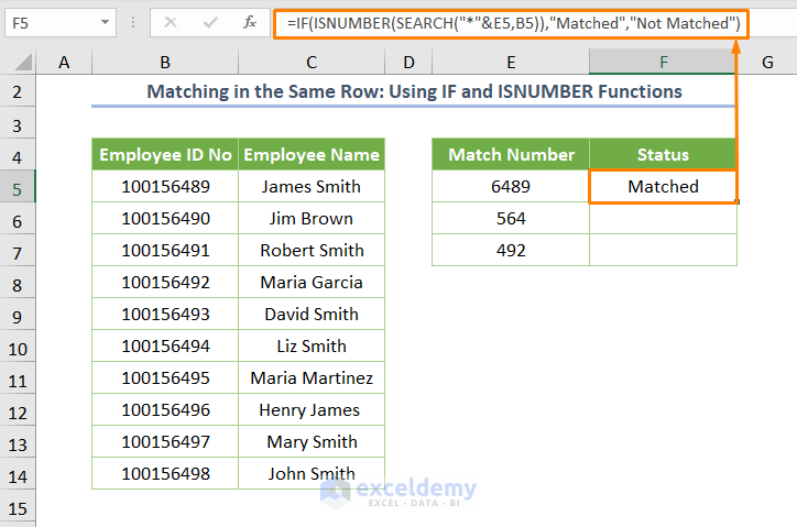
If you want to find the status either Matched or Not Matched in the same row, insert the following formula in the F5 cell and press ENTER.
=IF(ISNUMBER(SEARCH("*"&E5,B5)),"Matched","Not Matched")
Here, E5 is the starting cell of the Match Number and B5 is the starting cell of the Employee ID No.
⧬ In the above formula, the SEARCH function returns the position of a specific character inside the defined input. Here, the function finds “1” if the match number is matched with the Employee ID No. Else, it will return #VALUE! error. Then, the ISNUMBER function shows TRUE in the case of the matched output. Lastly, the IF function returns Matched instead of TRUE and Not Matched in the case of FALSE.
After using the Fill Handle tool (just drag down the cursor from the lower-right part of the F5 cell), you’ll get the following output.
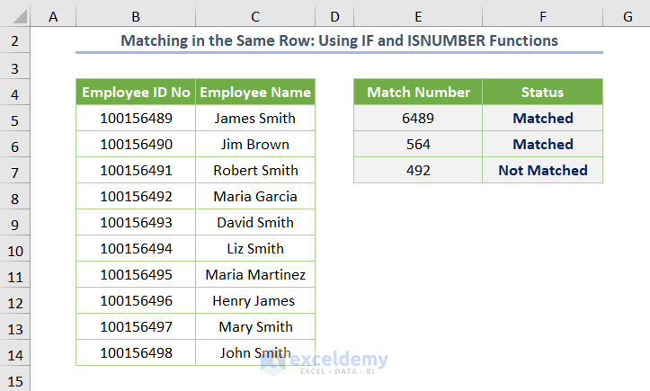
Have a deeper look at the output and you’ll notice that the F7 cell shows Not Matched though the match number is available in the B5:B14 cell range. It is because the match number doesn’t exist in the same row (in the B7 cell).
2. Utilizing MATCH and TEXT Functions
If you want to get the relative position of the numbers by performing the partial number match instead of getting the status in the first method, you may use the below formula.
=MATCH("*"&E5&"*",TEXT($B$5:$B$14,"0"),0)
Here, B5:B14 is the cell range representing the Employee ID No.
Note: This is an array formula, so press CTRL + SHIFT + ENTER if you’re not a Microsoft 365 user.
⧬ In the above formula, the TEXT function along with the “0” format code converts the number into text. Then, the MATCH function returns the relative position of the matched number. The A5:A14 cells show the relative position of the B5:B14 cells.
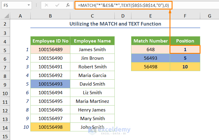
In the above image, the F5 cell shows “1” as the relative position of the B5 cell is 1.
3. INDEX-MATCH for Partial Number Match
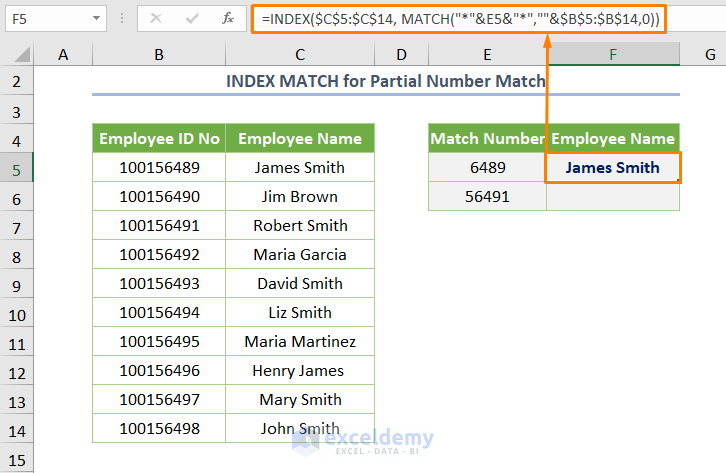
Furthermore, you may extract the cell value after executing the partial match against the numbers. So, use the below formula.
=INDEX($C$5:$C$14, MATCH("*"&E5&"*",""&$B$5:$B$14,0))
Here, C5:C14 cells refer to Employee Name.
⧬ In the above formula, the MATCH function returns the relative position based on the lookup value (e.g. E5 cell) from the B5:B14 cell range. Finally, the INDEX function extracts the cell value i.e. the name of the employee with respect to the matched Employee ID No.
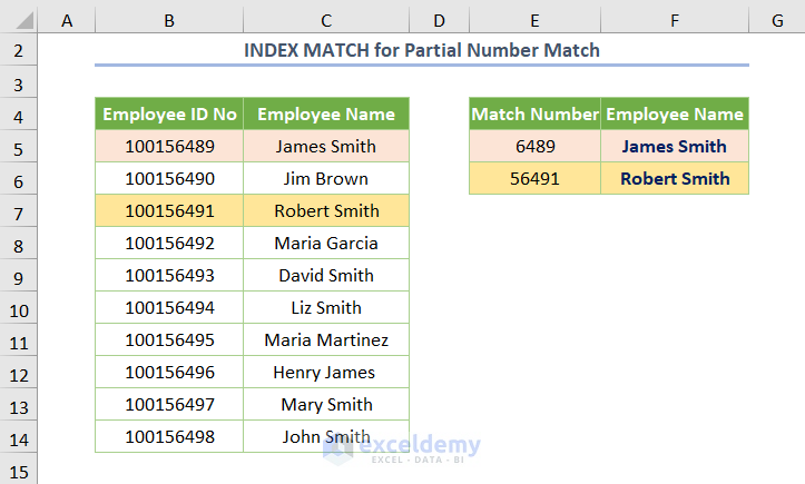
The rest output will be as follows.
4. Applying VLOOKUP Function
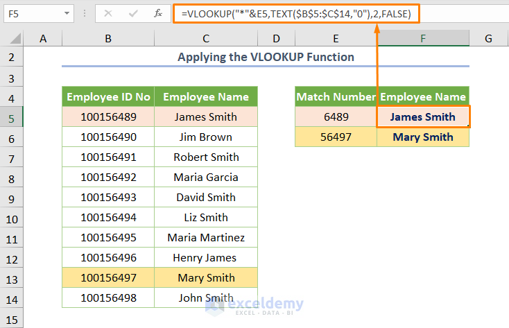
But if you are accustomed to using the VLOOKUP function, you may use the following formula for extracting the same output as found using the INDEX and MATCH functions.
=VLOOKUP("*"&E5,TEXT($B$5:$C$14,"0"),2,FALSE)
Here, B5:C14 is the table array converted into text, 2 is the col_index_num, and FALSE is for partial match.
⧬ If you want to skip the TEXT function, you can use the B5:C14 & “ “ as the table array.
5. Partial Number Match for Two Columns
Suppose, you want to perform the partial number match for two columns. The below screenshot shows Match Number1 in Column D and Match Number2 in Column E.
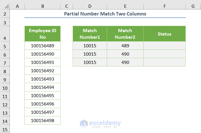
This can be executed in two ways.
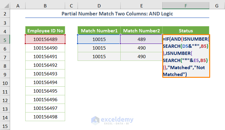
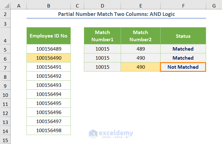
5.1. Using AND Logic
When you want to get the status e.g. “Matched” if the two Match Numbers return “Matched”. Simply, you can say the AND logic returns TRUE if all inputs are TRUE. Else, it will return FALSE.
=IF(AND(ISNUMBER(SEARCH(D5&"*",B5)),ISNUMBER(SEARCH("*"&E5,B5))),"Matched","Not Matched")
After inserting the formula and using the Fill Handle tool, you’ll get the following output.
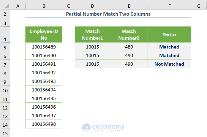
If you look closely at the following figure, you’ll find that the F7 cell shows Not Matched as the E7 cell doesn’t match with the B7 cell partially.
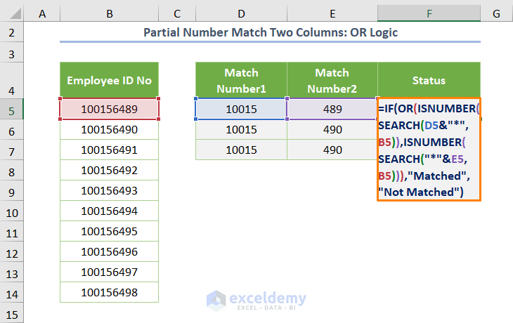
5.2. Using OR Logic
Again, you can apply the OR logic to return TRUE if any of the inputs are TRUE.
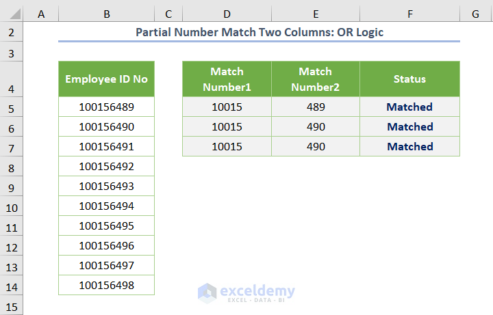
=IF(OR(ISNUMBER(SEARCH(D5&"*",B5)),ISNUMBER(SEARCH("*"&E5,B5))),"Matched","Not Matched")
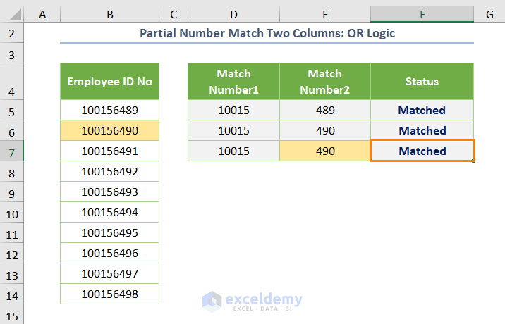
So, the output will be as follows.
In the below image, the F7 cell shows Matched because the D7 cell has a partial match with the B7 cell though the E7 cell doesn’t have that.
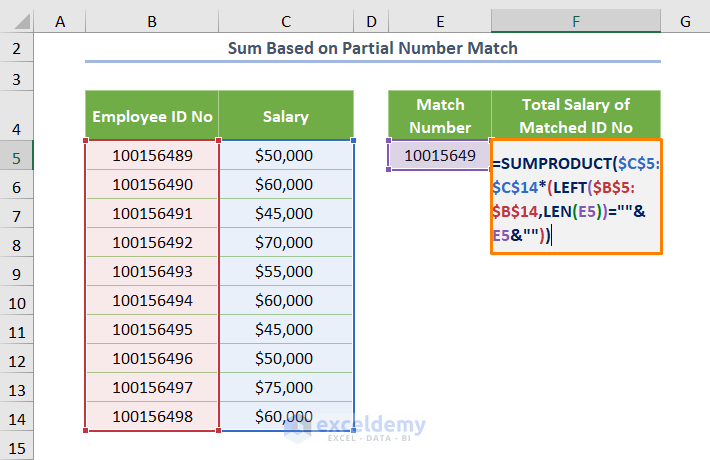
Sum Based on Partial Number Match
In addition, if you want to sum the value after performing the partial number match, you may use the following formula.
=SUMPRODUCT($C$5:$C$14*(LEFT($B$5:$B$14,LEN(E5))=""&E5&""))
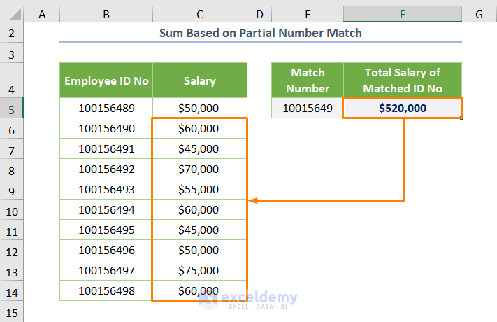
⧬ The LEFT function and the LEN function return TRUE if the Match Number matches with the Employee ID No. Lastly, the SUMPRODUCT function sums up the salary of the matched Employee ID No.
So, the output will be as follows.
Things to Remember
- While using the VLOOKUP or INDEX MATCH functions, you’ll get a #N/A error. If you want to avoid that you may use the IFERROR function.
- Asterisk (*) is used to perform the partial matching of either text or number.
Download Practice Workbook
Conclusion
That’s the end of today’s session. I strongly believe from now, you can easily perform the partial number match using the Excel formula. Anyway, if you have any queries or recommendations, please share them in the comments section.
<< Go Back to Partial Match Excel | Formula List | Learn Excel
Get FREE Advanced Excel Exercises with Solutions!
