Indeed, Microsoft Excel is a highly effective program. We can execute continuous operations on a given dataset using Excel’s tools and capabilities. Excel also offers an abundance of handy Library Functions. This article explains how Excel’s DELTA Function operates independently. In addition, we will examine three practical examples to have a better understanding of the DELTA Function. Therefore, you should go through these 3 practical examples to use DELTA Function in Excel.
Introduction to DELTA Function in Excel
- Summary
DELTA is a mathematical function in Excel that compares two numbers to see whether they are equal. DELTA yields 1 when the numbers are equivalent. Otherwise, DELTA returns 0.
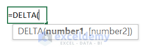
- Syntax
=DELTA(number1, [number2])
- Arguments
| ARGUMENT | REQUIRED/OPTIONAL | EXPLANATION |
|---|---|---|
| number1 | Required | The first number. |
| [number2] | Optional | The second number. If omitted, [number2] is assumed to be 0. |
- Version
All versions of Microsoft Excel have the DELTA function.
Using DELTA Function in Excel: 3 Practical Examples
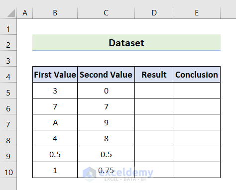
As an example, we shall investigate a sample dataset. For instance, the following dataset has four columns: First Value, Second Value, Result, and Conclusion. We will examine each practical case using the DELTA function in this post. In addition, I should have mentioned that I wrote this essay using Microsoft Excel 365. You can choose the version that best suits your needs.
1. Find Similar Values Between Two Columns Through DELTA Function
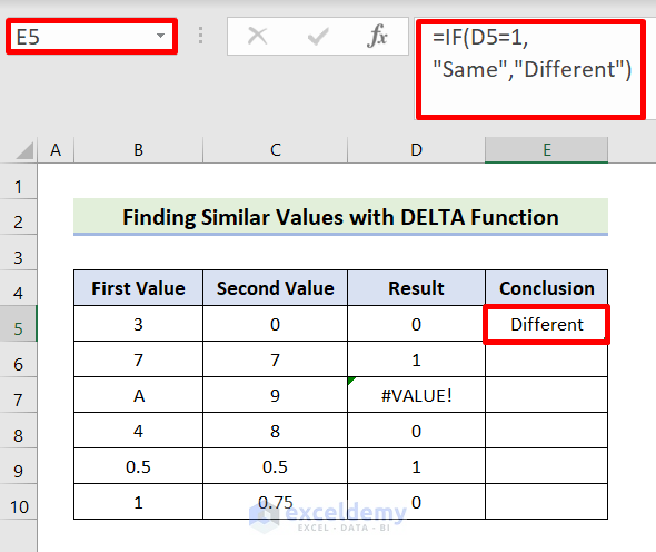
The first example of the DELTA function covered in this post is finding similar values in two columns. Here, the DELTA function compares the columns First Value and Second Value. The function returns 1 in the Result column if two values are identical. If not, DELTA returns 0. To facilitate comprehension, we illustrate a remark using the IF Function. Please follow these instructions attentively to complete the work.
STEPS:
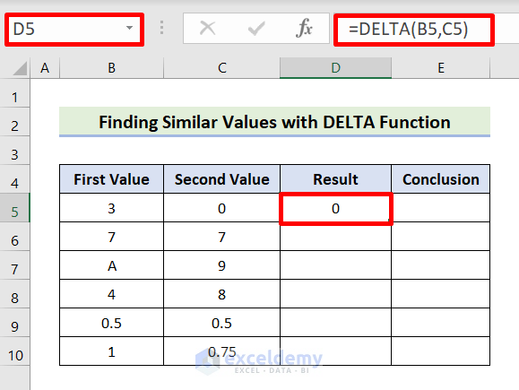
- First, select cell D5.
- Second, insert the following formula in D5.
=DELTA(B5,C5)- Later, hit the Tab key or Enter key.
- Subsequently, It provides the desired outcome as below.
- Apply the same method to other cells as was performed in cell D5.
- To get this, choose the Fill Handle icon.
- Importantly, hold and drag the Fill Handle icon to cell D10.
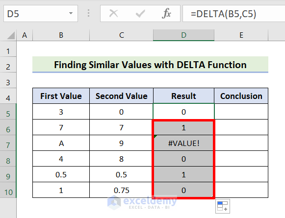
- Consequently, the required output will be returned, as seen below.
- We find a VALUE# error in cell D7 because one of our values is non-numeric. In this case, A in cell B7.
- At this point, choose cell E5.
- Then, write the below formula in cell E5.
=IF(D5=1,"Same","Different")- Now, hit Enter to see the intended outcome.
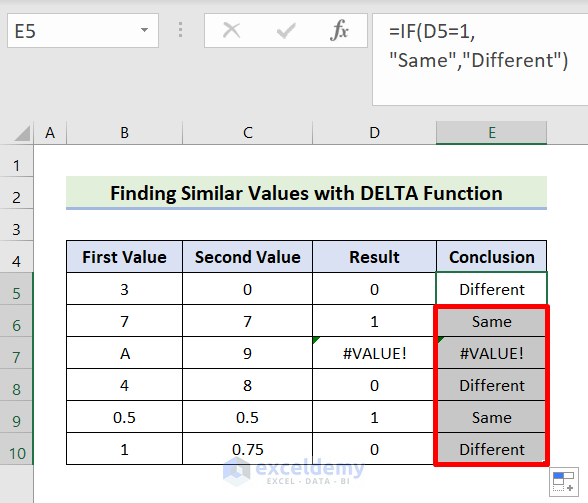
- Like previously, utilize the Fill Handle icon.
- Hold the icon and drag it to cell E10.
- Finally, we will find our desired output below.
- Due to the D7 cell, another VALUE# error will occur in E7.
2. Insert DELTA Function to Compare Column Values with 0
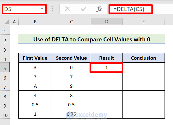
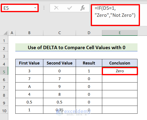
The second DELTA function demonstration in this tutorial compares cell values with 0. Here, the DELTA function compares the Second Value columns with zero. In this situation, only the Required parameter of the DELTA function will be provided. If the needed parameter is present, but the optional parameter is missing, DELTA assumes that the optional parameter is equal to 0. Using the IF function, we illustrate a remark for clarity. Therefore, carefully follow these instructions to complete the work.
STEPS:
- First of all, select cell D5.
- Later, insert the following formula into cell D5.
=DELTA(C5)- At this time, press Tab or Enter at a later time.
- Thus, it yields the intended effect, as seen below:
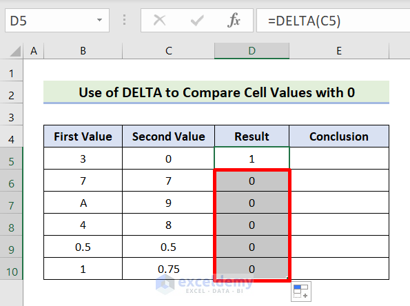
- Next, apply the same procedure to other cells as was done with cell D5.
- Now, use the Fill Handle symbol to get this.
- Importantly, Not only hold but also move it to the D10 cell.
- As a result, the needed output will be returned, as seen below.
- At this time, choose cell E5.
- Enter the following formula in cell E5:
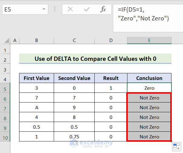
=IF(D5=1,"Zero","Not Zero")- Now, press Enter to see the desired result.
- As before, utilize the Fill Handle symbol.
- Significantly move the sign to cell E10 while holding it down.
- At last, it will show the required result below.
Read More: How to Calculate Delta in Excel
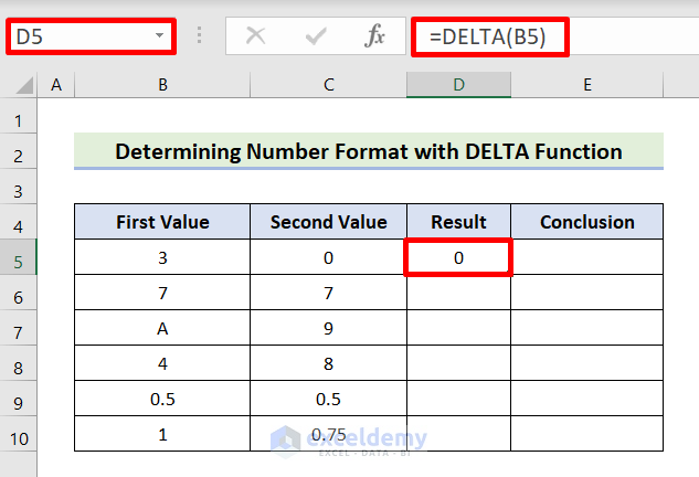
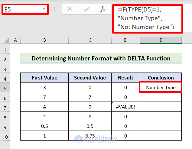
3. Utilize DELTA Function to Determine Number Format in Excel
In this part of the study of the DELTA function, we will also examine another practical and appealing case. We can identify whether the value of a cell is a number. Here, we will use the DELTA function to determine if the First Value column has numeric values. To be highly involved, we illustrate a message in the Conclusion column using the TYPE Function. So, follow these steps below attentively to complete the work.
STEPS:
- To begin, select the D5 cell first.
- Second, input the formula below into cell D5.
=DELTA(B5)- At this moment, hit Tab or Enter to proceed.
- Consequently, it has the desired effect, as seen below.
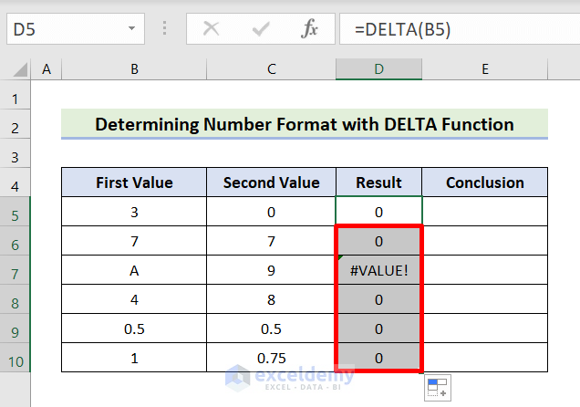
- Afterward, repeat the same method to other cells as was done with cell D5.
- Presently, use the Fill Handle icon to get this.
- Importantly, hold the Fill Handle icon and drag it to cell D10.
- The relevant output will be returned, as seen below.
- At this stage, choose cell E5.
- Then, type the formula below into cell E5.
=IF(TYPE(D5)=1,"Number Type","Not Number Type")- Now, press Enter to see what you want to happen.
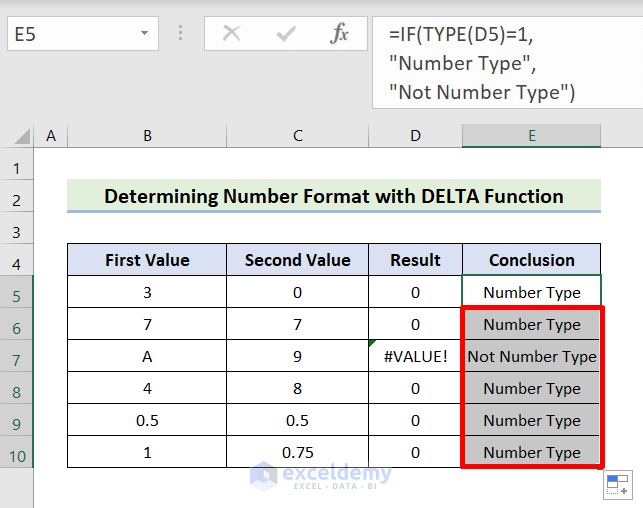
- After that, use the Fill Handle symbol as you did before.
- Importantly, hold the icon down and move it to cell E10.
- Last but not least, the output we want is shown below.
Read More: How to Calculate Delta Percentage in Excel
Common Errors While Using Excel DELTA Function
| Common Errors | When They Show |
|---|---|
| #VALUE! | When number 1 or [number2] does not have a numeric value, #VALUE! Error appears. |
Download Practice Workbook
Obtain a free copy of the example workbook used during the session.
Conclusion
After learning about the DELTA Function and seeing how it works in the examples we discussed, you can now use it in Excel. Keep using this and let us know if you think of other ways to get the work done or if you have any new ideas. Remember to leave questions, comments, or suggestions in the section below.
Excel DELTA Function: Knowledge Hub
<< Go Back to Excel Functions | Learn Excel
Get FREE Advanced Excel Exercises with Solutions!
