What Is Delta E?
Here, E represents “Empfindung”. Actually, Empfindung is a German word that means sensation. On the other hand, Delta is a Greek word that meand the gradual change of a variable. So, Delta E represents changes in sensation.
You can measure Delta E on a scale from 0 to 100. 0 meaning less color difference and 100 full distortion. Perception ranges explained by Zachary Schuessler are Shown below:
- <= 1.0: Imperceptible to the human eye.
- 1-2: distinguishable through close attention.
- 2-10: Perceptible at first sight.
- 11-49: Colors are comparable to the opposite.
- 100: Colors are definitely the opposite.
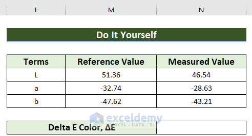
The sample dataset showcases Terms, Reference Value, and Measured Value.
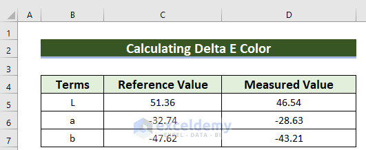
L, a, and b represent three axes of color.
- L represents darkness (0) to lightness (100).
- a means shades of greenness (-128) to redness (+127).
- b means shades of blueness (-128) to yellowness (+127).
Method 1 – Using a Generic Formula to Compute Delta E Color
Steps:
- Select a blank cell D9 to keep Delta E Color.
- Enter this formula in D9.
=((C5-D5)^2+(C6-D6)^2+(C7-D7)^2)^(1/2)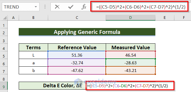
- Press ENTER to see the result.

Read More: How to Calculate Delta in Excel
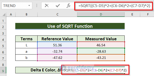
Method 2 – Using the Excel SQRT Function for Delta E Color Calculation
Steps:
- Select a blank cell D9 to keep Delta E Color.
- Enter this formula in D9.
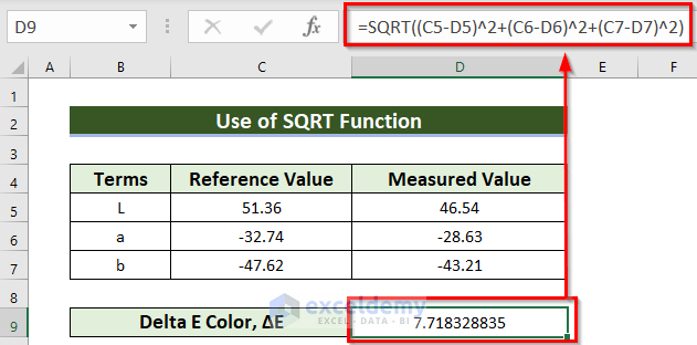
=SQRT((C5-D5)^2+(C6-D6)^2+(C7-D7)^2)The SQRT function will return the square root of the summation of three terms (the square of subtraction from reference value to measured value).
- Press ENTER.
- This is the output.
Read More: How to Calculate Option Greek Delta in Excel
Method 3 – Merge the SQRT & POWER Functions to Calculate Delta E
Steps:
- Select a blank cell D9 to keep Delta E Color.
- Enter this formula in D9.
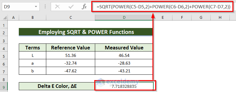
=SQRT(POWER(C5-D5,2)+POWER(C6-D6,2)+POWER(C7-D7,2))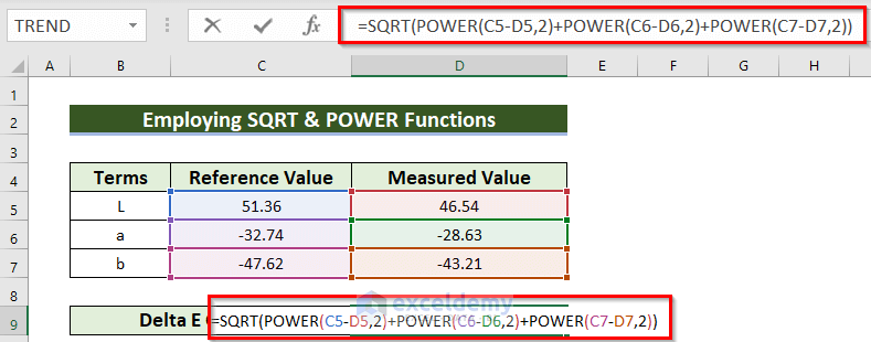
Formula Breakdown
- The POWER function will return the output of a number raised to a specified power.
- POWER(C7-D7,2)—> the subtraction of a measured value (D7) from the reference value (C7) is base, 2 is the specified power.
- Output: 19.4481.
- POWER(C6-D6,2)—> returns 16.8921.
- POWER(C5-D5,2)—> turns 23.2324.
- The Plus sign (+) adds the three outputs.
- Output: 59.5726.
- The SQRT function returns the square root.
- Press ENTER.
- This is the output.
Read More: How to Calculate Delta Delta CT in Excel
Method 4 – Combining the SQRT & SUMSQ Functions to Find Delta E Color
Steps:
- Select a blank cell D9 to keep Delta E Color.
- Enter this formula in D9.
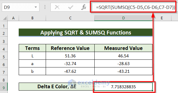
=SQRT(SUMSQ(C5-D5,C6-D6,C7-D7))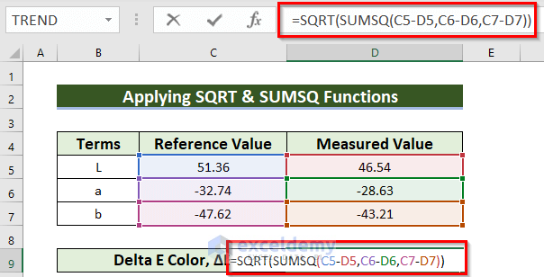
Formula Breakdown
- The SUMSQ function returns the summation of the square of three terms (the subtraction from the reference value to the measured value).
- SUMSQ(C5-D5,C6-D6,C7-D7)—> returns 59.5726.
- The SQRT function returns the square root.
- Press ENTER to see the result.
Practice Section
Practice the methods.
Download Practice Workbook
You can download the practice workbook from here:
Related Articles
- How to Calculate Delta Percentage in Excel
- Delta Neutral Strategy in Excel
- Delta Hedging Example in Excel
- How to Calculate VaR Using Delta-Normal Method in Excel
<< Go Back to Excel DELTA Function | Excel Functions | Learn Excel
Get FREE Advanced Excel Exercises with Solutions!

Very helpful, and big thank you for the excel sheet.
I use to give an free program to my students,taking from a printing company that gives the small program for free.
But this is more helpful.
Thanks from Portugal
Hello Jose,
You are most welcome. Your appreciation means a lot to us.
Regards
ExcelDemy
you dont make clear this is DE from 1976 formulation. Todays industry standard is DE 2000.
Hello,
Thank you for pointing that out! Yes, the method shown in the article uses the ΔE from the 1976 (CIE76) formulation.
You are correct that the current industry standard is ΔE 2000 (CIEDE2000), which provides a more accurate measure of color difference.
For advanced applications, it’s better to use the DE 2000 calculation.
Regards
ExcelDemy
Do you have the Delta E: CIE 2000? for xls
Hello KK,
The article currently demonstrates Delta E using the CIE76 method only.
CIEDE2000 (Delta E 2000) is more complex and requires several intermediate calculations.
However, CIEDE2000 can be implemented in Excel by adding extra columns for the intermediate steps or by using a single Excel 365 formula.
Regards,
ExcelDemy