Microsoft Excel is a powerful software. We can perform numerous operations on our datasets using Excel tools and features. There are many default Excel functions that we can use to create formulas. Many educational institutions and business companies use Excel files to store valuable data. Sometimes, we estimate possible outcomes from real-life projects. Accordingly, recording those probable scenarios in an Excel worksheet is necessary. In that case, we can stay prepared for whatever happens. Hence, this article will show you the step-by-step procedures to create a scenario with changing cells in Excel.
How to Create a Scenario with Changing Cells in Excel: Easy Steps
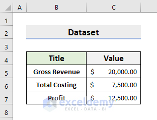
In real life, we predict certain outcomes. And we prepare a strategy for each case. Therefore, it can be effective if we record the probable scenarios in an Excel worksheet. To illustrate, we’ll use a sample dataset as an example. For instance, the following dataset has Gross Revenue and Total Costing. In cell C8, we have the Profit (Gross Revenue – Total Costing). Here, we’ll create 3 Scenarios (Minimum Case, Average Case, Maximum Case) where the cells C5 and C6 will change the values according to each scenario. Now, go through the steps carefully to perform the task.
STEP 1: Use Scenario Manager
- First, select Data ➤ Forecast ➤ What-If Analysis ➤ Scenario Manager.

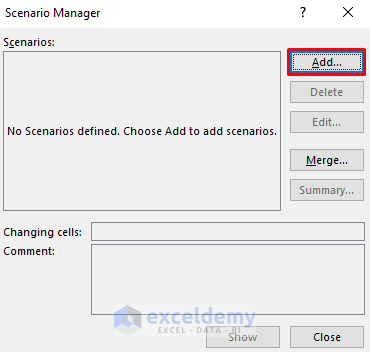
- Consequently, the Scenario Manager dialog box will pop out.
- Click Add.
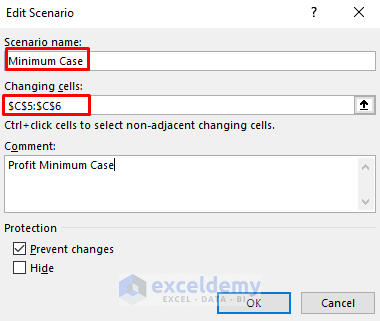
- Another dialog box will appear.
- There, type Minimum Case in the Scenario name.
- Choose cells C5 and C6 in the Changing cells.
- Then, input any desired Comment.
- Afterward, press OK.
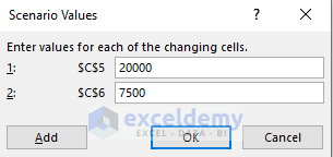
- Subsequently, the Scenario Values dialog box will emerge.
- In this example, we’ll keep the original values in the Minimum Case scenario.
- You can input any values you want.
- After that, press Add to create another scenario.
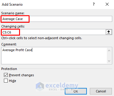
- Thus, the Add Scenario dialog box will pop out.
- Type Average Case in the Scenario name.
- Select cells C5 and C6 in the Changing cells.
- Input any desired Comment.
- Then, press OK.
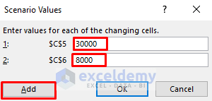
- The Scenario Values dialog box will appear.
- Insert 30000 for cell C5 and 8000 for cell C6.
- Again, press Add to create the Maximum Case.
- Repeat the above steps as necessary.
Read More: How to Use Scenario Manager in Excel
STEP 2: View Scenario Summary
- Now, we’ll generate the scenario summary.
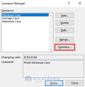
- For this purpose, go to Data ➤ Forecast ➤ What-If Analysis ➤ Scenario Manager.
- In the pop-out dialog box, press Summary.
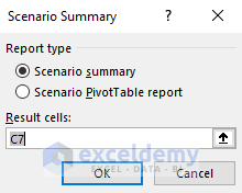
- Next, check the circle for the Scenario Summary.
- Then, press OK.
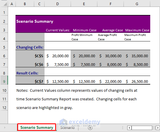
- Thus, you’ll get a new worksheet named Scenario Summary.
- There, you’ll see all the cases and the values.
Read More: How to Create a Scenario Summary Report in Excel
STEP 3: Place Scenario Tab to Excel Ribbon
However, it’ll be efficient to add Scenario to Excel Ribbon in case you want to see the scenarios in your original sheet. So, learn the process.
- Firstly, right-click on the Data tab.
- Then, select Customize the Ribbon.

- Hence, it’ll return the following dialog box.
- There, choose All Commands.
- Next, select Data Tools in the Data section.
- Press New Group.

- After that, click the New Group.
- Press Rename.

- In the Rename dialog box, Type Scenario in the Display name.
- Press OK.

- Subsequently, select the Scenario command in the left-side pane.
- Click Add.

- Thus, it’ll return a new Scenario ribbon in the Data tab.
- From now on, it’ll be easier to switch between different scenarios.

Download Practice Workbook
Download the following workbook to practice by yourself.
Conclusion
Henceforth, you will be able to create a scenario with changing cells in Excel following the above-described procedures. Keep using them and let us know if you have more ways to do the task. Don’t forget to drop comments, suggestions, or queries if you have any in the comment section below.
Related Articles
- How to Create Scenarios in Excel
- Scenario Analysis in Excel
- How to Edit Scenarios in Excel
- How to Remove Scenario Manager in Excel
<< Go Back to Excel What-If Analysis Scenario Manager | What-If Analysis in Excel | Learn Excel
Get FREE Advanced Excel Exercises with Solutions!
