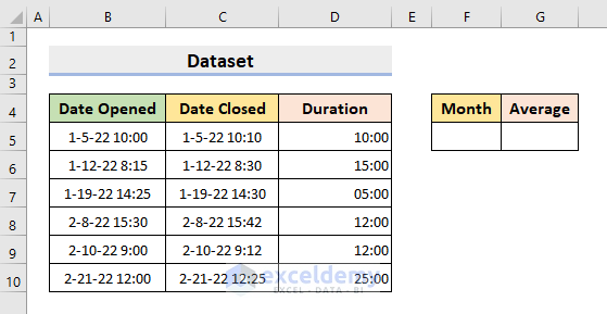
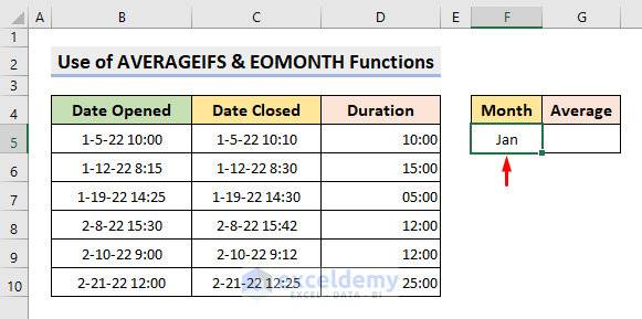
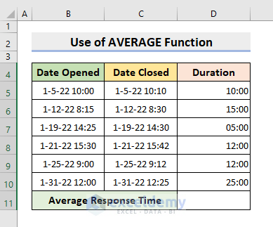
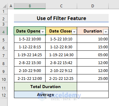
The following dataset represents the order placement date and time: Date Opened, Date Closed, and Duration of a courier firm.
How to Calculate the Average Response Time in Excel: 4 Methods
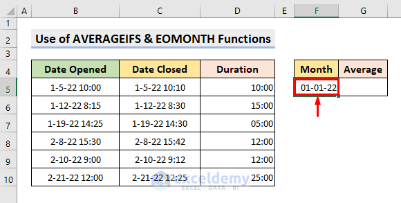
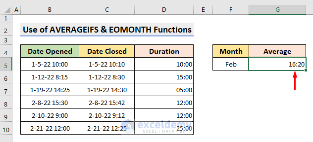
Method 1 – Use Excel AVERAGEIFS and EOMONTH Functions to Calculate Average Response Time
STEPS:
- Select cell F5.
- Insert 01-01-22.
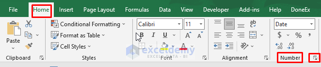
- Select the drop-down icon in the Number group under the Home tab.
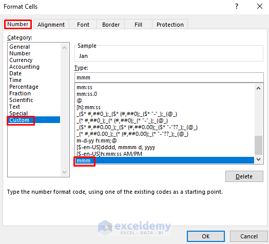
- The Format Cells dialog box will appear.
- Select ‘mmm’ in the Custom Type under the Number tab to see the F5 cell value in month names.
- Press OK.
- You’ll see ‘Jan’ in cell F5.
- Select cell G5.
- Insert this formula:
=AVERAGEIFS(D5:D10,B5:B10,">=" & F5,B5:B10,"<=" & EOMONTH(F5,0))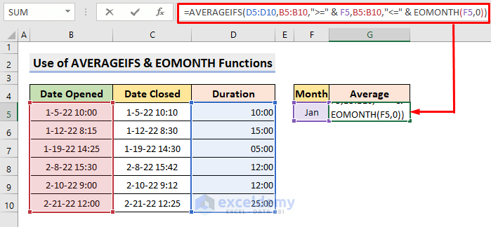
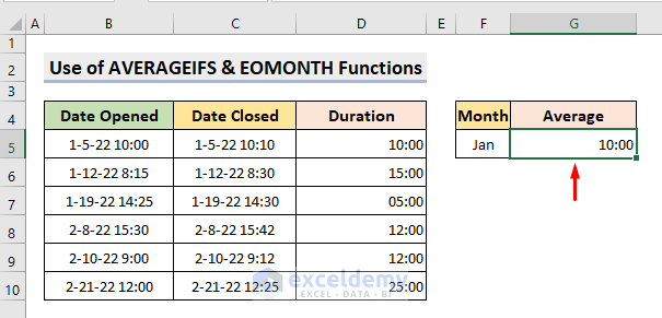
- Press Enter. The average response time for January will appear in cell G5.
How Does the Formula Work?
- EOMONTH(F5,0)
This looks for the last date of the same month given in cell F5 as we have placed 0 in the second argument of this formula.
- AVERAGEIFS(D5:D10,B5:B10,”>=” & F5,B5:B10,”<=” & EOMONTH(F5,0))
This entire formula computes the average. Here, ‘D5:D10’ is the range for calculating the average. ‘B5:B10’ is the criteria range. Our first criterion is to match the dates that are greater or equal to the first day of January. Our second criterion is to match the dates that are less or equal to the last day of January.
If you want to calculate the average response time in February follow the steps.
STEPS:
- In cell F5, insert 01-02-2022.
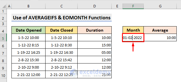
- The updated result will appear in cell G5.
Read More: How to Calculate Average Turnaround Time in Excel
Method 2 – Average Response Time Calculation with the Excel AVERAGE Function
We’ll use the same dataset.
STEPS:
- Select cell D11.
- Insert the following:
=AVERAGE(D5:D10)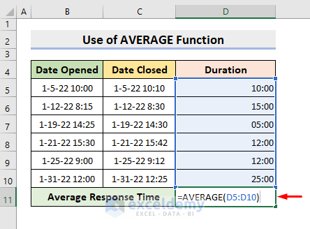
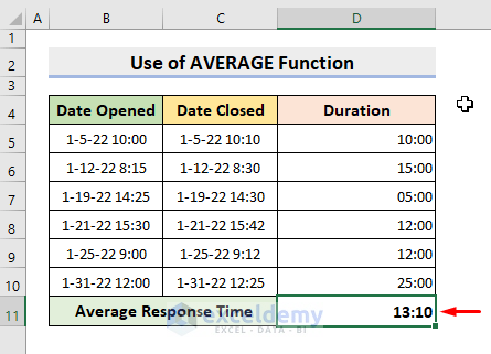
- Press Enter.
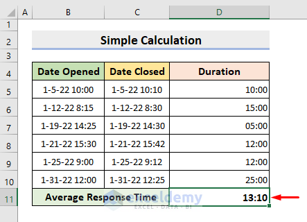
Method 3 – Calculate the Average Response Time Manually in Excel
STEPS:
- Select cell D11 and insert:
=SUM(D5:D10)/6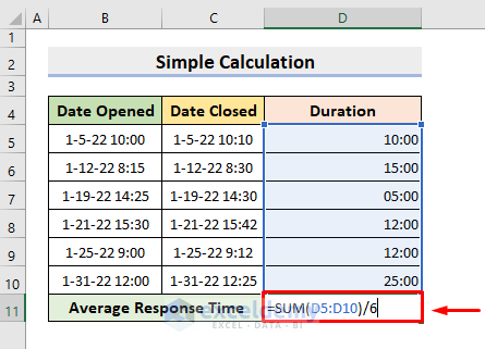
- Press Enter.
Related Content: How to Calculate Average Handling Time in Excel
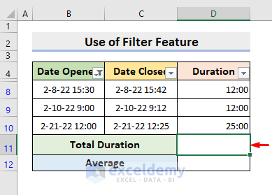
Method 4 – Apply the Excel Filter Feature to Calculate the Average Response Time
The Filter feature takes a specified month into account only.
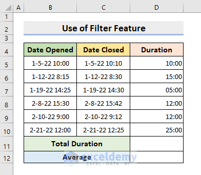
STEPS:
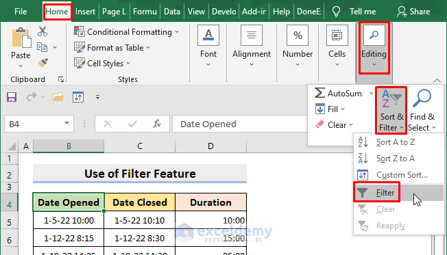
- Select cell B4.
- Select Filter from the Sort & Filter drop-down list in the Editing group under the Home tab.
- You’ll see the data table like it’s shown below.
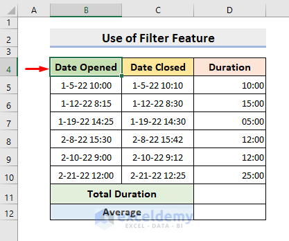
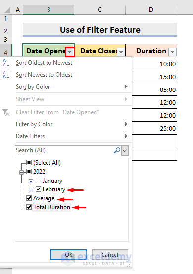
- Select the drop-down icon for the Date Opened column. Check February, Average, and Total Duration.
- Press OK.
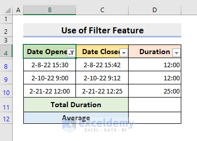
- The table will contain only the inputs for February.
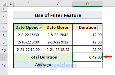
- Select cell D11.
- Select the AutoSum feature in the Editing group under the Home tab and press Enter.
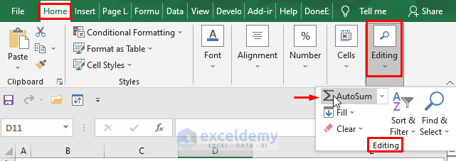
- The sum will appear in cell D11.
- Select cell D12.
- Insert this formula:
=D11/COUNT(B8:B10)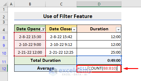
- Press Enter and it’ll return the precise result.
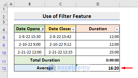
The COUNT function counts the total number of inputs from B8 to B10. You’ll need to modify the range if the values aren’t sorted.
Download the Practice Workbook
Related Articles
- How to Calculate Elapsed Time in Excel
- How to Calculate Cycle Time in Excel
- How to Calculate Turnaround Time in Excel Excluding Weekends
- How to Calculate Years of Service in Excel
- How to Calculate Turnaround Time in Excel
<< Go Back to Calculate Average Time | Calculate Time | Date-Time in Excel | Learn Excel
Get FREE Advanced Excel Exercises with Solutions!
