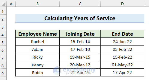
We have the following dataset which contains the Employee Name, Joining Date, and End Date of employees. We will calculate the Years of Service for them.
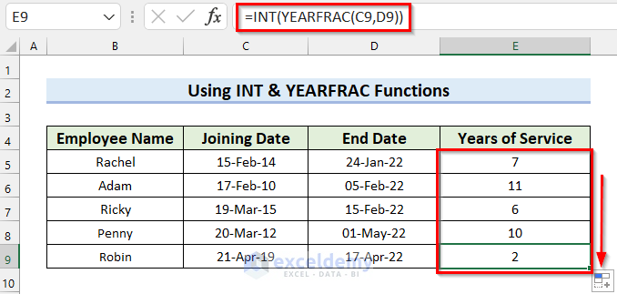
Method 1 – Combining Excel INT anf YEARFRAC Functions to Calculate the Years of Service
Steps:
- Select the cell where you want to calculate the Years of Service. We selected cell E5.
- Insert the following formula:
=INT(YEARFRAC(C5,D5))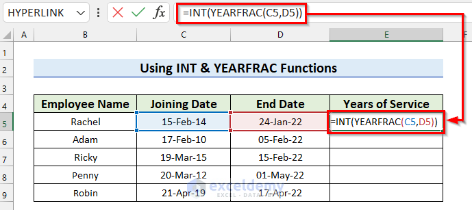
Formula Breakdown
- YEARFRAC(C5,D5) —-> The YEARFRAC function will return a fraction of the year represented by the number of days between the dates in cells C5 and D6.
- Output: 7.94166666666667
- INT(YEARFRAC(C5,D5)) —-> turns into
- INT(7.94166666666667) —-> The INT function will return the integer number by rounding it down.
- Output: 7
- INT(7.94166666666667) —-> The INT function will return the integer number by rounding it down.
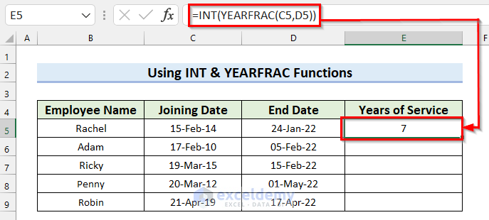
- Press Enter to get the result.
- Drag the Fill Handle down to copy the formula to the other cells.
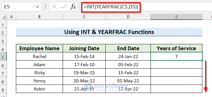
- Here’s our result.
Related Content: How to Calculate Elapsed Time in Excel
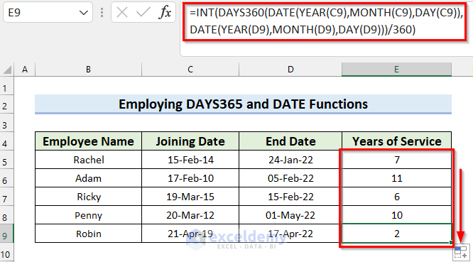
Method 2 – Joining DAYS360 and DATE Functions in Excel to Calculate the Years of Service
Steps:
- Select the cell where you want to calculate the Years of Service. We selected cell E5.
- Use the following formula in it:
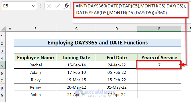
=INT(DAYS360(DATE(YEAR(C5),MONTH(C5),DAY(C5)),DATE(YEAR(D5),MONTH(D5),DAY(D5)))/360) 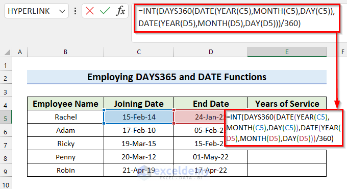
Formula Breakdown
- DAY(D5) —-> The DAY function will return the day number of the date in cell D5.
- Output: 24
- MONTH(D5) —-> \The MONTH function will return the month number of the given date in cell D5.
- Output: 1
- YEAR(D5) —-> The YEAR function will return the year number of the given date in cell D5.
- Output: 2022
- DATE(YEAR(D5),MONTH(D5),DAY(D5)) —-> turns into
- DATE(2022,1,24) —-> The DATE function will return a serial number that represents a date from a given year, month, and day.
- Output: 44585
- DATE(2022,1,24) —-> The DATE function will return a serial number that represents a date from a given year, month, and day.
- DATE(YEAR(C5),MONTH(C5),DAY(C5)) —-> turns into
- DATE(2014,2,15) —-> The DATE function will return a serial number that represents a date from a given year, month, and day.
- Output: 41685
- DATE(2014,2,15) —-> The DATE function will return a serial number that represents a date from a given year, month, and day.
- DAYS360(DATE(YEAR(C5),MONTH(C5),DAY(C5)),DATE(YEAR(D5),MONTH(D5),DAY(D5))) —-> turns into
- DAYS360(41685,44585) —-> The DAYS360 function will return the number of days between the two given dates.
- Output: 2859
- DAYS360(41685,44585) —-> The DAYS360 function will return the number of days between the two given dates.
- INT(DAYS360(DATE(YEAR(C5),MONTH(C5),DAY(C5)),DATE(YEAR(D5),MONTH(D5),DAY(D5)))/360) —-> turns into
- INT(2859/360) —-> The INT function will return the integer number by rounding it down.
- Output: 7
- INT(2859/360) —-> The INT function will return the integer number by rounding it down.
- Press Enter to get the result.
- Drag the Fill Handle to copy the formula to the other cells.
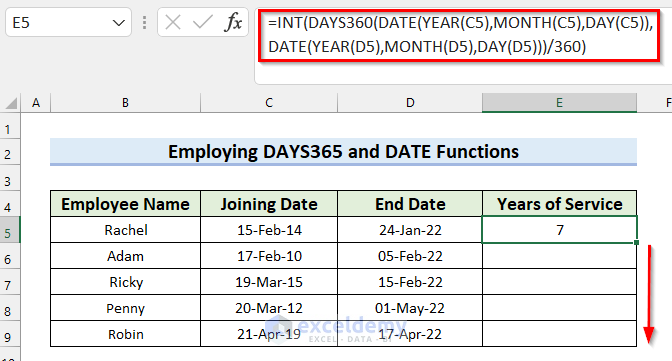
- Here’s our result.
Method 3 – Using the DATEDIF Function to Calculate the Years of Service in Excel
Case 3.1 – Applying the DATEDIF Function to Calculate Years
Steps:
- Select the cell where you want to calculate the Years of Service. We selected cell E5.
- Insert the following formula.
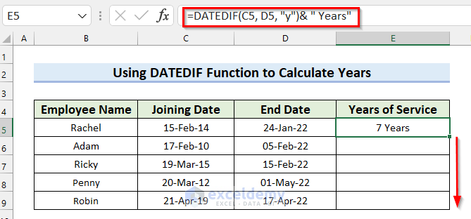
=DATEDIF(C5, D5, "y")& " Years"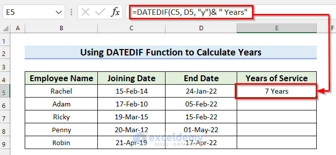
Formula Breakdown
- DATEDIF(C5, D5, “y”) —-> The DATEDIF function will return the number of years between the two given dates.
- Output: 7
- DATEDIF(C5, D5, “y”)& ” Years” —-> turns into
- 7& ” Years” —-> The Ampersand (&) operator will combine the text and formula.
- Output: “7 Years”
- 7& ” Years” —-> The Ampersand (&) operator will combine the text and formula.
- Hit Enter.
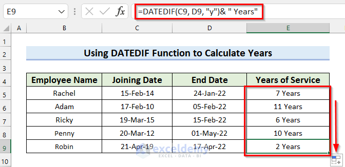
- Drag the Fill Handle down to copy the formula.
- Here are our results.
Case 3.2 – Using the DATEDIF Function to Calculate Years and Months
Steps:
- Select the cell where you want to calculate the Years of Service. We selected cell E5.
- Insert the following formula:
=DATEDIF(C5,D5,"y")&" Years, "&DATEDIF(C5,D5,"ym")&" Months"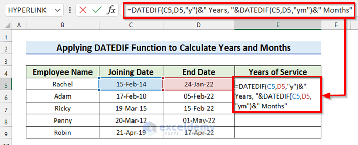
Formula Breakdown
- DATEDIF(C5,D5,”y”) —-> The DATEDIF function will return the number of years between the two given dates.
- Output: 7
- DATEDIF(C5,D5,”ym”) —-> The DATEDIF function will return the number of months between the two given dates ignoring the days and years.
- Output: 11
- DATEDIF(C5,D5,”y”)&” Years, “&DATEDIF(C5,D5,”ym”)&” Months” —-> turns into
- 7&” Years, “&11&” Months” —-> The Ampersand (&) operator will combine the texts and formulas.
- Output: “7 Years, 11 Months”
- 7&” Years, “&11&” Months” —-> The Ampersand (&) operator will combine the texts and formulas.
- Press Enter to get the result.

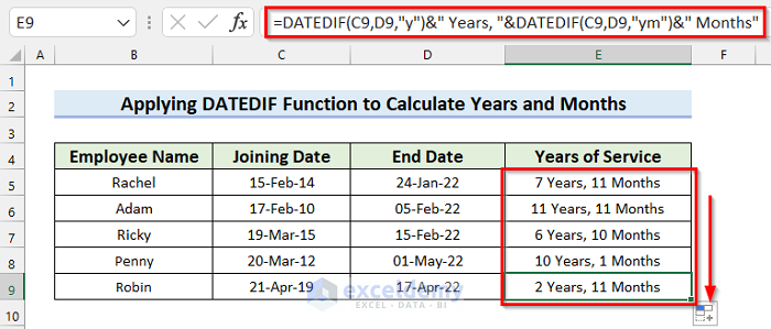
- Drag the Fill Handle down to copy the formula.
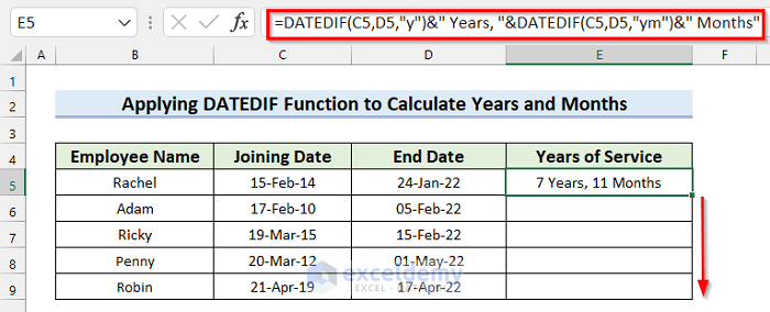
- Here are our results.
Case 3.3 – Inserting the DATEDIF Function to Calculate Years, Months, and Days
Steps:
- Select the cell where you want to calculate the Years of Service. We selected cell E5.
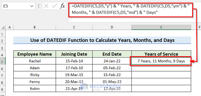
- Insert the following formula:
=DATEDIF(C5,D5,"y") & " Years, " & DATEDIF(C5,D5,"ym") & " Months, " & DATEDIF(C5,D5,"md") & " Days"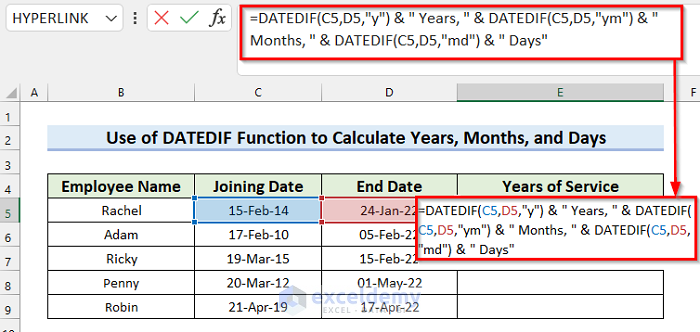
Formula Breakdown
- DATEDIF(C5,D5,”y”) —-> The DATEDIF function will return the number of years between the two given dates.
- Output: 7
- DATEDIF(C5,D5,”ym”) —-> The DATEDIF function will return the number of months between the two given dates ignoring the days and years.
- Output: 11
- DATEDIF(C5,D5,”md”) —-> The DATEDIF function will return the number of days between the two given dates ignoring the months and years.
- Output: 9
- DATEDIF(C5,D5,”y”) & ” Years, ” & DATEDIF(C5,D5,”ym”) & ” Months, ” & DATEDIF(C5,D5,”md”) & ” Days” —-> turns into
- 7 & ” Years, ” & 11 & ” Months, ” & 9 & ” Days” —-> The Ampersand (&) operator will combine the texts and formulas.
- Output: “7 Years, 11 Months, 9 Days”
- 7 & ” Years, ” & 11 & ” Months, ” & 9 & ” Days” —-> The Ampersand (&) operator will combine the texts and formulas.
- Press Enter to get the result.
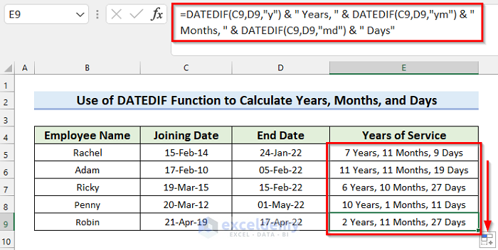
- Drag the Fill Handle down to copy the formula.
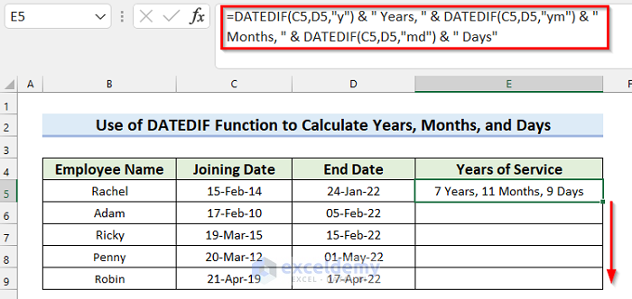
- Here are our results.
Method 4 – Merging Excel IF and DATEDIF Functions to Calculate Service Years
Case 4.1 – Returning a Text String If the Service Duration Is Less Than One Year
Steps:
- Select the cell where you want to calculate the Years of Service. We selected cell E5.
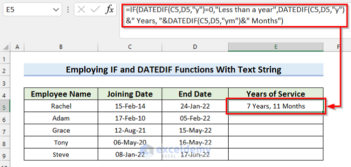
- Insert the following formula:
=IF(DATEDIF(C5,D5,"y")=0,"Less than a year",DATEDIF(C5,D5,"y")&" Years, "&DATEDIF(C5,D5,"ym")&" Months")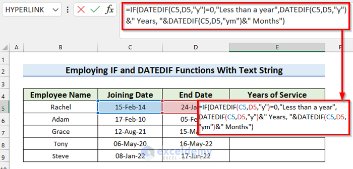
Formula Breakdown
- DATEDIF(C5,D5,”y”) —-> The DATEDIF function will return the number of years between the two given dates.
- Output: 7
- DATEDIF(C5,D5,”ym”) —-> The DATEDIF function will return the number of months between the two given dates ignoring the days and years.
- Output: 11
- IF(DATEDIF(C5,D5,”y”)=0,”Less than a year”,DATEDIF(C5,D5,”y”)&” Years, “&DATEDIF(C5,D5,”ym”)&” Months”) —-> turns into
- IF(7=0,”Less than a year”,7&” Years, “&11&” Months”) —-> The IF function will check the logical_test. If it is True, the formula will return “Less than a year”. If it is False, the formula will return the Years of Service in years and months.
- Output: “7 Years, 11 Months”
- IF(7=0,”Less than a year”,7&” Years, “&11&” Months”) —-> The IF function will check the logical_test. If it is True, the formula will return “Less than a year”. If it is False, the formula will return the Years of Service in years and months.
- Press Enter to get the result.
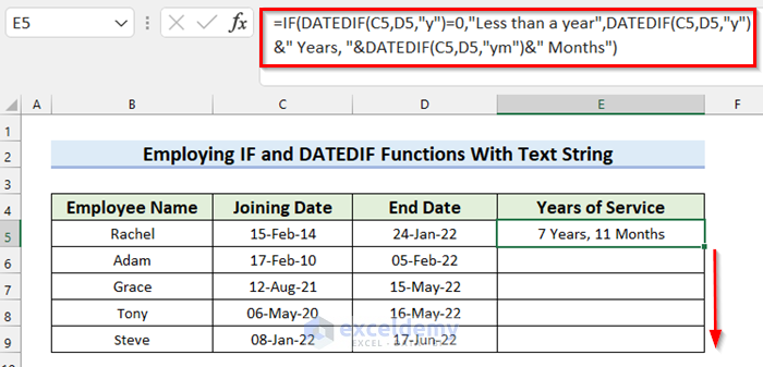
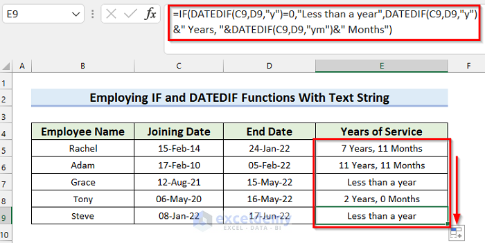
- Drag the Fill Handle to copy the formula.
- Here are our results.
Case 4.2 – Calculating the Month If the Service Duration Is Less Than One Year
Steps:
- Select the cell where you want to calculate the Years of Service. We selected cell E5.
- Insert the following formula:
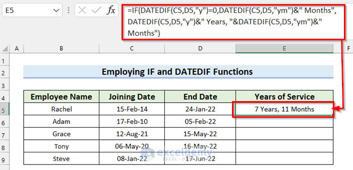
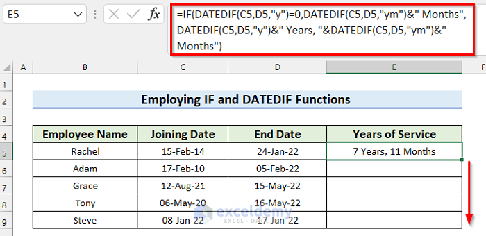
=IF(DATEDIF(C5,D5,"y")=0,DATEDIF(C5,D5,"ym")&" Months",DATEDIF(C5,D5,"y")&" Years, "&DATEDIF(C5,D5,"ym")&" Months")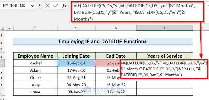
Formula Breakdown
- DATEDIF(C5,D5,”y”) —-> The DATEDIF function will return the number of years between the two given dates.
- Output: 7
- DATEDIF(C5,D5,”ym”) —-> This DATEDIF function will return the number of months between the two given dates ignoring the days and years.
- Output: 11
- IF(DATEDIF(C5,D5,”y”)=0,DATEDIF(C5,D5,”ym”)&” Months”,DATEDIF(C5,D5,”y”)&” Years, “&DATEDIF(C5,D5,”ym”)&” Months”) —-> turns into
- IF(7=0,11&” Months”,7&” Years, “&11&” Months”) —-> The IF function will check the logical_test. If it is True, the formula will return the Years of Service in months. If it is False, the formula will return the Years of Service in years and months.
- Output: “7 Years, 11 Months”
- IF(7=0,11&” Months”,7&” Years, “&11&” Months”) —-> The IF function will check the logical_test. If it is True, the formula will return the Years of Service in months. If it is False, the formula will return the Years of Service in years and months.
- Press Enter to get the result.
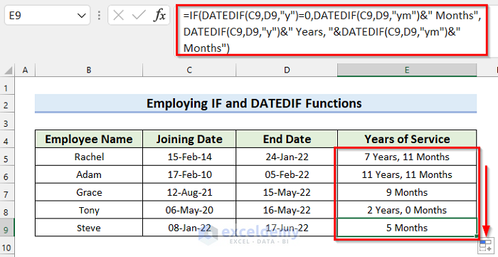
- Drag the Fill Handle to copy the formula.
- Here are our results.
Calculate the Years of Service in Excel from the Hire Date to Now in Excel
Steps:
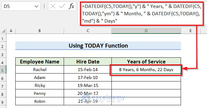
- Select the cell where you want to calculate the Years of Service. We selected cell D5.
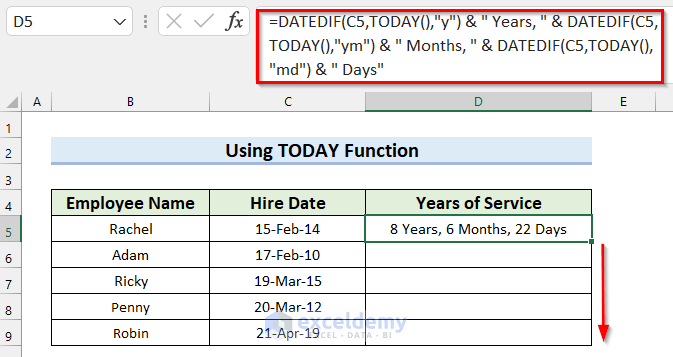
- Insert the following formula:
=DATEDIF(C5,TODAY(),"y") & " Years, " & DATEDIF(C5,TODAY(),"ym") & " Months, " & DATEDIF(C5,TODAY(),"md") & " Days"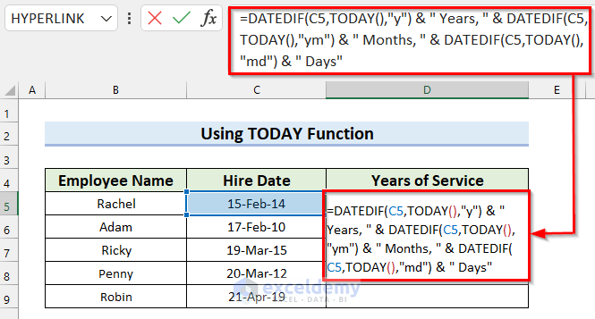
Formula Breakdown
- DATEDIF(C5,TODAY(),”y”) —-> The DATEDIF function will return the number of years between the Hire Date and the Current Date.
- Output: 8
- DATEDIF(C5,TODAY(),”ym”) —-> The DATEDIF function will return the number of months between the Hire Date and the Current Date ignoring the days and years.
- Output: 6
- DATEDIF(C5,TODAY(),”md”) —-> The DATEDIF function will return the number of days between the Hire Date and the Current Date ignoring the months and years.
- Output: 22
- DATEDIF(C5,TODAY(),”y”) & ” Years, ” & DATEDIF(C5,TODAY(),”ym”) & ” Months, ” & DATEDIF(C5,TODAY(),”md”) & ” Days” —-> turns into
- 8 & ” Years, ” & 6 & ” Months, ” & 22 & ” Days” —-> The Ampersand (&) operator will combine the texts and formulas.
- Output: “8 Years, 6 Months, 22 Days”
- 8 & ” Years, ” & 6 & ” Months, ” & 22 & ” Days” —-> The Ampersand (&) operator will combine the texts and formulas.
- Press Enter to get the result.
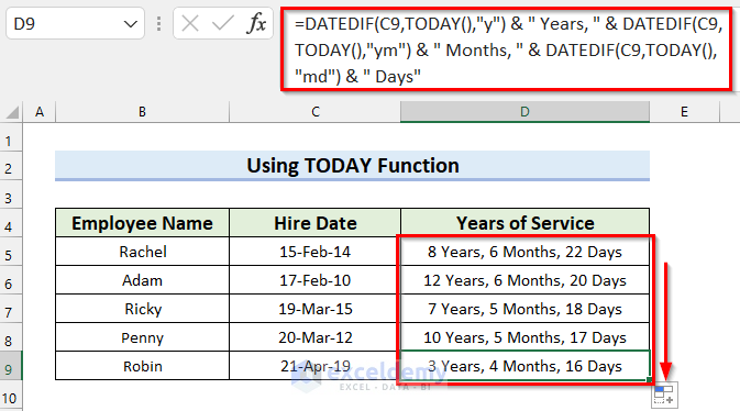
- Drag the Fill Handle to copy the formula.
- Here are our results.
Read More: How to Calculate Cycle Time in Excel
Calculating the End Date from the Hire Date after Certain Years of Service
Steps:
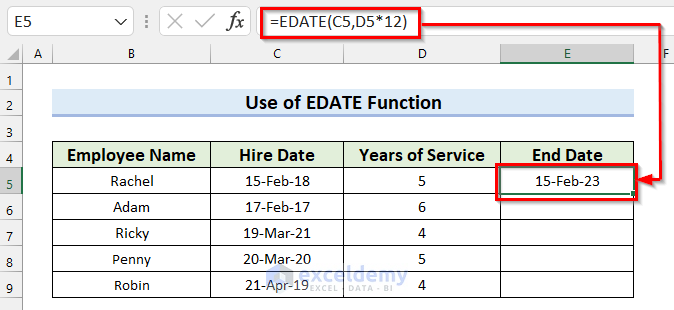
- Select the cell where you want to calculate the End Date. We selected cell E5.
- Insert the following formula:
=EDATE(C5,D5*12) 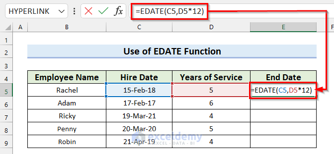
In the EDATE function, we selected C5 as start_date and D5*12 as months. We multiplied the years by 12 to convert them into months. The formula will return the date after these selected months.
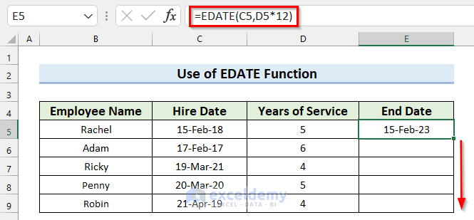
- Press Enter, and you will get the End Date.
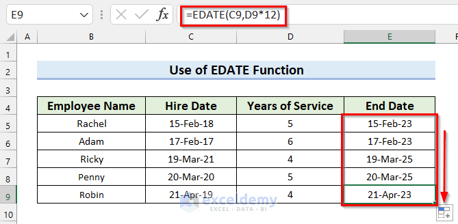
- Drag the Fill Handle to copy the formula.
- Here’s our results.
Download the Practice Workbook
Related Articles
- How to Calculate Turnaround Time in Excel Excluding Weekends
- How to Calculate Turnaround Time in Excel
- How to Calculate Average Handling Time in Excel
- How to Calculate Average Response Time in Excel
- How to Calculate Average Turnaround Time in Excel
<< Go Back to Calculate Total Time | Calculate Time | Date-Time in Excel | Learn Excel
Get FREE Advanced Excel Exercises with Solutions!

Very useful formula for HR Professionals.
Thanks Chamila for your feedback!
This was very helpful! Great information! Thank you very much!
Thanks so much! This made things a whole lot easier for me. As Chamila said, very useful formula for HR folks.
Thanks for your feedback, LuluBelle! Glad to know that it helped.
This formula has a bug. If you input joining date of 01/01/20, and a present date of 31/12/20, it returns 0years, 11 Months, 30 Days. However this is actually 1 year, 0 months and 0 days.
Hi Justin,
Thanks for notifying this. I will check and update the article.
Regards
I want to subscribe
THANK YOU VERY MUCH for sharing!