Method 1 – Compute the Average Turnaround Time in Excel
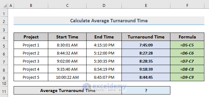
Look at the following picture. We have the Start Time and the End Time of some Projects. With those values, we extracted the Turnaround Time for our dataset. We will get the Average Turnaround Time for our dataset in Excel.
Steps:
- Pick the result cell to store the Average Turnaround Time (in our case, it is Cell E11).
- Insert the following formula:
=AVERAGE(E5:E9)Here,
E5:E9 = Range of the Turnaround Times to calculate the Average.
- Press Enter.

Read More: How to Calculate Average Handling Time in Excel
Method 2 – Estimate Average TAT in DATE Format
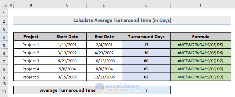
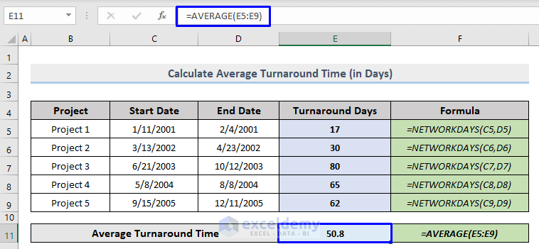
You can see in the picture shown below that we have provided the formulas that were applied to get the Turnaround Days for our dataset in Column F. We will see how to get the Average Turnaround value of those data.
Steps:
- Pick the result cell to store the Average Turnaround Time (in our case, it is Cell E11).
- Insert the following formula:
=AVERAGE(E5:E9)Here,
E5:E9 = Range of the Turnaround Times to calculate the Average.
- Press Enter.
Read More: How to Calculate Average Response Time in Excel
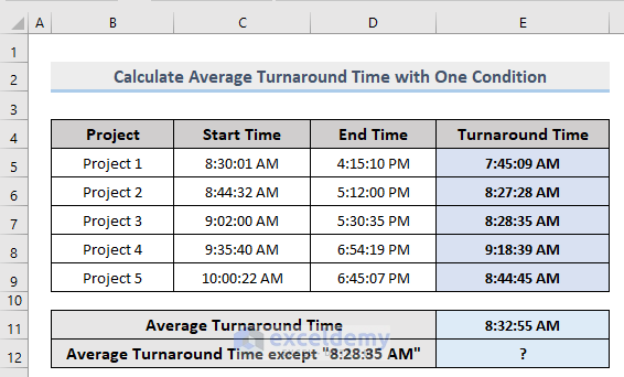
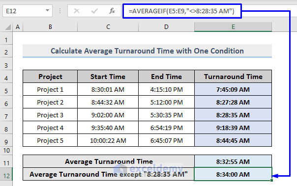
Method 3 – Compute the Average Turnaround Time with One Condition in Excel
This time we will compute the Average Turnaround Time while excluding one specific value from our dataset. We will exclude “8:28:35 AM” from the values.
Steps:
- Select the result cell (in our case, it is Cell E12).
- Insert the following formula:
=AVERAGEIF(E5:E9,"<>8:28:35 AM")Here,
- E5:E9 = Range of the Turnaround Times to calculate the Average.
- “<>8:28:35 AM” = Value to exclude
- Press Enter.
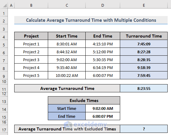
Method 4 – Calculate the Average Turnaround Time with Multiple Conditions
We will calculate the Average Turnaround Time between the times that are greater than or equal to the Start Time “9:02:00 AM” and less than or equal to the End Time “6:00:07 PM” in our dataset. We have stored “9:02:00 AM” in Cell D14 and “6:00:07 PM” in Cell D15 in our Excel spreadsheet.
Steps:
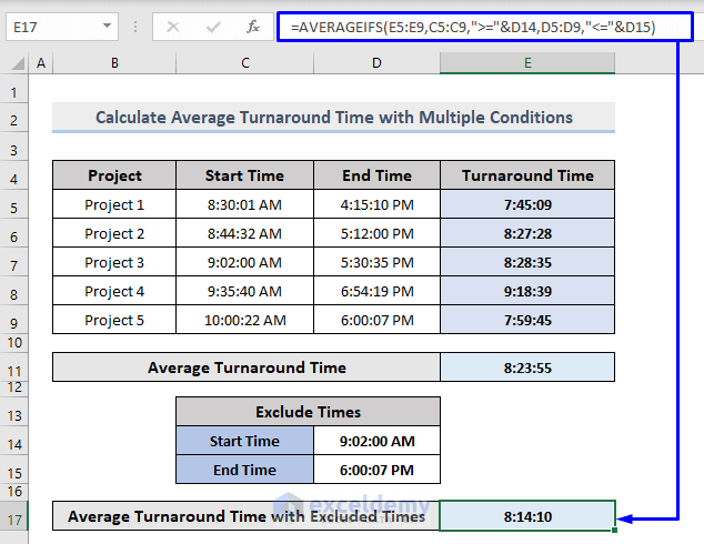
- Select the result cell (in our case, it is Cell E17).
- Insert the following function:
=AVERAGEIFS(E5:E9,C5:C9,">="&D14,D5:D9,"<="&D15)Here,
- E5:E9 = Range of the Turnaround Times to calculate the Average
- C5:C9 = Range of the Start Times
- D14 = The specific Start Time to exclude
- D5:D9 = Range of the End Times
- D14 = The specific End Time to exclude
- Press Enter.
Download the Workbook
Related Articles
- How to Calculate Elapsed Time in Excel
- How to Calculate Cycle Time in Excel
- How to Calculate Turnaround Time in Excel Excluding Weekends
- How to Calculate Years of Service in Excel
<< Go Back to Calculate Average Time | Calculate Time | Date-Time in Excel | Learn Excel
Get FREE Advanced Excel Exercises with Solutions!

can i use manually holiday during in NETWORKDAYS.INTL. For example i have every Sunday and third and fourth of every month Saturday are holiday.
Hello KARAN
Thanks for reaching out and posting such an interesting comment. Yes, you can manually specify holidays using the NETWORKDAYS.INTL function to customize which days are considered weekends and also lets you include specific holidays.
In your case, the first and second arguments in the formula are for the start and end dates; you can use 11 3rd arguments to consider only Sunday as the weekend. In the 4th argument, you insert the specified holiday.
I have developed a formula for January by focusing on your specified weekends and holidays.
Hopefully, the formula will help; good luck.
Regards
Lutfor Rahman Shimanto
ExcelDemy