The string from which characters will be extracted. It can be any text value, number, or array.
start_num
Required
The starting position from which characters will be extracted. It can be a single number or an array of numbers.
num_chars
Required
The total number of characters that will be extracted. It can be a single number or an array of numbers.
Note:
The first argument text can be any text value, number, or array of text values or numbers. But whether it is a text value or a number, the return value will always be a text value.
The next two arguments start_num and num_chars can be any number or an array of numbers.
If you use an array argument, the formula will be an Array Formula, and you have to press Ctrl + Shift + Enter.
Return Value:
Returns a text value consisting of a specific number of characters starting from a specific position of a string.
Special Notes:
If the start_num argument is greater than the total number of characters of a string, the MID function will return an empty string.
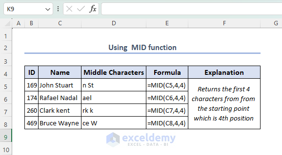
Now, we will see the MID function in action.
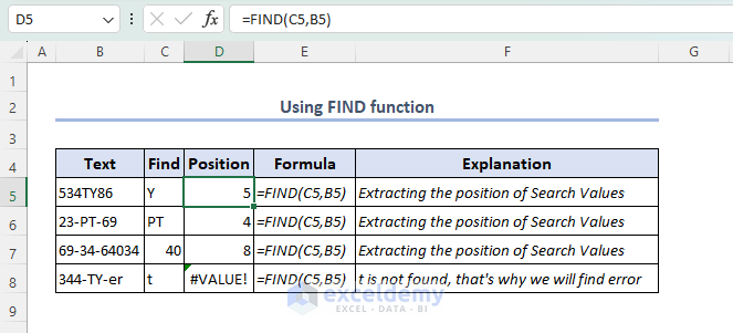
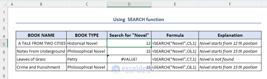
Function 5 – SEARCH Function
The SEARCH function returns the number of characters after finding a specific character or text string, reading from left to right. This function Searches for a case-insensitive match. It works for both Array and Non-Array Formula and is available from Excel 2003.
Syntax:
The syntax of the SEARCH function is:
SEARCH(find_text,within_text,[start_num])
Arguments:
ARGUMENT
REQUIREMENT
EXPLANATION
find_text
Required
The text that is searched for. It can be a single text or an array of texts.
within_text
Required
The text value within which the find_text argument is searched for. It can be a single text value or an array of text values.
[start_num]
Optional
The position of the within_text argument from which it starts searching. It can be a single number or an array of numbers. The default is 1.
Note:
All three arguments can be either a single value or an array of values.
If at least one of the arguments is an array, the formula will become an Array Formula, and you must press Ctrl + Shift + Enter to enter it.
The third argument [start_num] is optional. The default is 1.
Return Value
Returns the number of characters at which the specific character or text string (find_text) is first found, reading from left to right.
We get the dataset showing how the SEARCH function works.
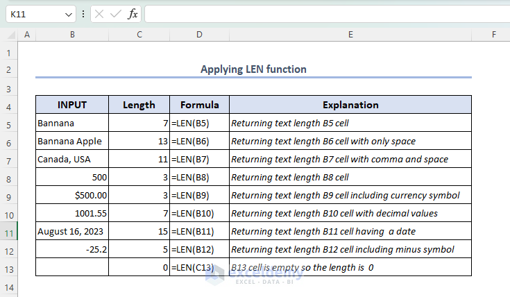
Function 6 – LEN Function
The LEN function in Excel returns the length of a given string. It is useful for a variety of purposes, including finding the number of characters in a given cell or range of cells or in a given string of text.
Syntax:
The LEN function is described with the following syntax:
=LEN(TEXT)
Arguments:
Argument
Required or Optional
Value
text
Required
The text for which to calculate length.
Note:
LEN reflects the length of text as a number.
This function works with numbers, but number formatting is not included.
LEN function returns zero in terms of empty cells.
We will see the LEN function in action.
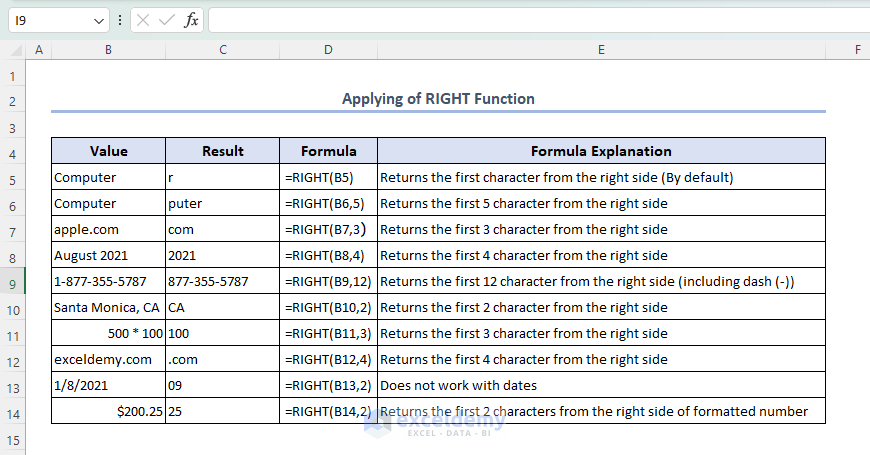
Function 7 – RIGHT Function
Syntax:
=RIGHT(text,[num_chars])
Arguments Explanation:
Arguments
Required/Optional
Explanation
text
Required
Pass the text from which to extract characters on the right.
[num_chars]
Optional
Pass the number of characters to extract, starting on the right. The default value is 1.
Version:
The RIGHT function is available from Excel 2007 to the latest version.
Notes
If num_chars is not provided, it defaults to 1.
If num_chars is greater than the number of characters available, the RIGHT function returns the entire text string.
RIGHT will extract digits from numbers as well as text.
This function does not consider the formatting of any cell, like a date, currency, etc.
While writing this article, I’m using the Office 365.
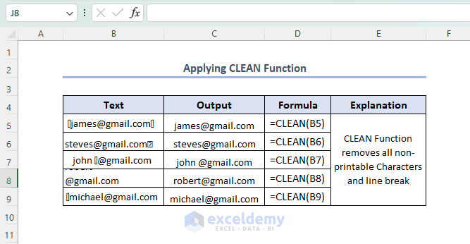
After entering the function, it will give you the text string free from all non-printable characters.
Note:
The CLEAN function can only remove the non-printable characters represented by numbers 0 to 31 in the 7-bit ASCII code.
Finally, we see the various instances of using the CLEAN function.
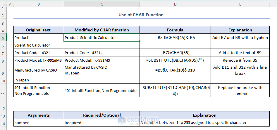
Function 11 – CHAR Function
Syntax:
=CHAR(number)
Argument Explanation:
Argument
Required/Optional
Explanation
number
Required
A number between 1 to 255 is assigned to a specific character
Return Parameter:
The CHAR function will return a character based on the number given as an argument.
Now, we see the output of the CHAR function in different instances.
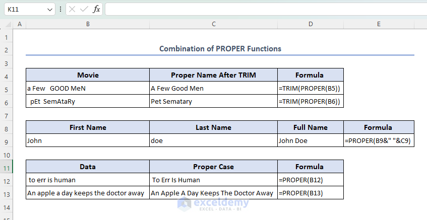
Function 12 – PROPER Function
Usually, the PROPERfunction converts a text string into the proper case, the first letter in each word to uppercase, and all other letters to lowercase.
Syntax:
=PROPER(text)
Arguments:
Argument
Required/Optional
Explanation
text
Required
The text should be converted to a proper case. The text could, however, be a formula that yields text, text surrounded in quotation marks, or perhaps a reference to such a cell that includes the text.
Returning Parameter:
It returns the first letter of every word to uppercase and other letters to lowercase.
Now, we finally see the PROPER function in action.
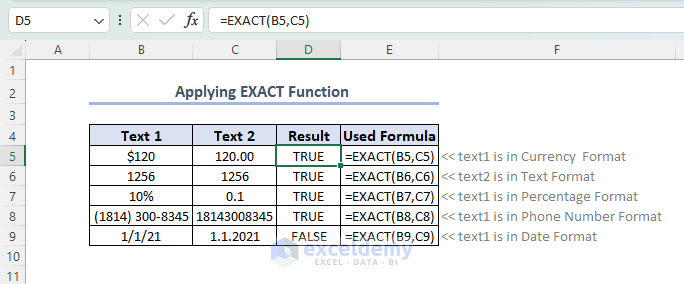
Function 13 – EXACT Function
The EXACT function compares two texts and then returns TRUE (in case the texts are exactly the same) or FALSE (in case they are not exactly the same).
Syntax:
=EXACT (text1,text2)
Arguments Explanation:
Arguments
Required/Optional
Explanation
text1
Required
First text string
text1
Required
Second text string
Return Parameter:
TRUE or FALSE, depending on the exact match between the two arguments.
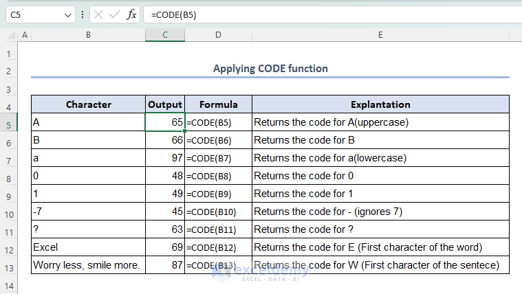
For any text string, a code will be returned for the first character of the text string
Return Parameter:
A numeric number will be returned for the first character of the input text string. In general, the number returned by CODE represents the ASCII decimal code for a character. The CODE function was developed to operate in an ASCII/ANSI domain, and it only knows how to map characters to integers 0-255.
Data Truncation: When using functions like LEFT, RIGHT, or MID to extract a portion of a text string, there’s a risk of data truncation if the specified length exceeds the actual length of the text. This can result in missing or incomplete information.
Case Sensitivity Issues: Excel String Functions are generally case-sensitive. If there’s a mismatch in the text being compared or manipulated, the results may not be as expected, leading to errors or incorrect outputs.
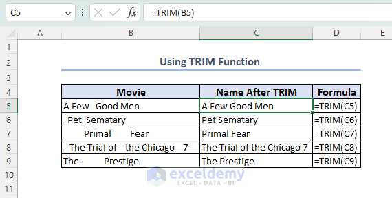
Leading and Trailing Spaces: Extra leading or trailing spaces in text strings can cause discrepancies in search, comparison, and data manipulation operations. Functions like TRIM can be used to address this, but if overlooked, it can lead to issues
Joyanta Mitra, a BSc graduate in Electrical and Electronic Engineering from Bangladesh University of Engineering and Technology, has dedicated over a year to the ExcelDemy project. Specializing in programming, he has authored and modified 60 articles, predominantly focusing on Power Query and VBA (Visual Basic for Applications). His expertise in VBA programming is evident through the substantial body of work he has contributed, showcasing a deep understanding of Excel automation, and enhancing the ExcelDemy project's resources with valuable... Read Full Bio