Overview: Excel SUMIF Function
- Objective:
The function adds the cells specified by a given condition or criteria.
- Formula:
=SUMIF(range, criteria, [sum_range])
- Arguments:
range- The range of cells where the condition will be applied.
criteria- Condition for the selected range of cells.
[sum_range]- The range of cells where the outputs are lying.
For more detailed explanations and examples with the SUMIF function, click here.
Overview: Excel VLOOKUP Function
- Objective:
The VLOOKUP function looks for a value in the leftmost column in a table and then returns a value in the same row from a specified column.
- Formula:
=VLOOKUP(lookup_value, table_array, col_index_num, [range_lookup])
- Arguments:
lookup_value- The value which it looks for in the leftmost column of the given table. Can be a single value or an array of values.
table_array- The table in which it looks for the lookup_value in the leftmost column.
col_index_num- The number of the column in the table from which a value is to be returned.
[range_lookup]- Tells whether an exact or partial match of the lookup_value is required. 0 for an exact match, 1 for a partial match. Default is 1 (partial match).
Method 1 – Combining SUMIF with VLOOKUP to Find Matches and Sum in the Same Excel Worksheet
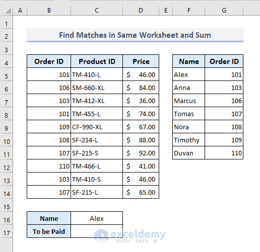
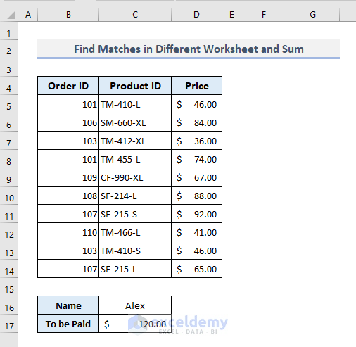
The first table (B4:D14) represents some random order data with product IDs and their corresponding prices. The second table on the right shows the customer names and their IDs. We’ll search for a specific customer name present in cell C16, fetch the orders for the corresponding customer, and make a sum of the total price to be paid in cell C17.
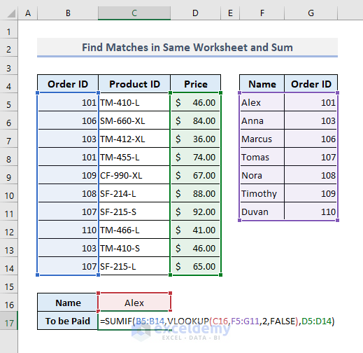
- In the output Cell C17, the required formula with the SUMIF and VLOOKUP functions will be:
=SUMIF(B5:B14,VLOOKUP(C16,F5:G11,2,FALSE),D5:D14)
- After pressing Enter, you’ll get the return value as shown in the picture below.
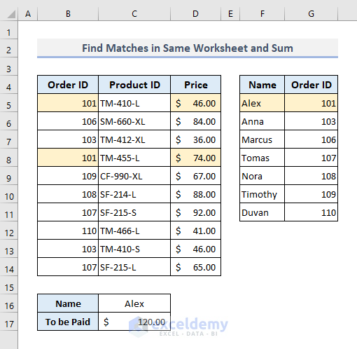
How Does the Formula Work?
- In this formula, the VLOOKUP function works as the second argument (Criteria) of the SUMIF function.
- The VLOOKUP function looks for the name Alex in the lookup array (F5:G11) and returns the ID number for Alex.
- Based on the ID number found in the previous step, the SUMIF function adds up all the prices for the corresponding ID number.
Read More: How to Vlookup and Sum Across Multiple Sheets in Excel
Method 2 – Joining SUMIF with VLOOKUP to Find Matches and Sum in Different Worksheets
The lookup array or table is present in another worksheet (Sheet2). The following worksheet (Sheet1) contains the primary data with the output cell.

Here’s the second worksheet (Sheet2), where the lookup array is present.
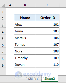
To include the above lookup array in the VLOOKUP function, we have to mention the worksheet name (Sheet2).
- Use this formula in the output Cell C17:
=SUMIF(B5:B14,VLOOKUP(C16,Sheet2!B3:C9,2,FALSE),Sheet1!D5:D14)

- Press Enter, and you’ll get the resulting value.
Read More: VLOOKUP and Return All Matches in Excel
Method 3 – Combining VLOOKUP, SUMPRODUCT, and SUMIF Functions for Multiple Excel Sheets
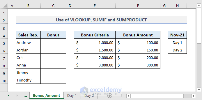
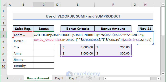
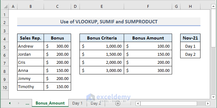
We’ll make a sum from the data available in different two different worksheets and then extract a value with the VLOOKUP function based on the corresponding amount of the sum. In the picture below, the worksheet named Bonus_Amount is present with 3 different tables. The leftmost table will show the sales bonuses for the corresponding sales representatives. We have to extract these bonus amounts by applying the VLOOKUP function for the array (E5:F8) related to the bonus criteria. The bonus criteria is actually the total sales which we have to pull from two different worksheets named ‘Day 1’ and ‘Day 2’.
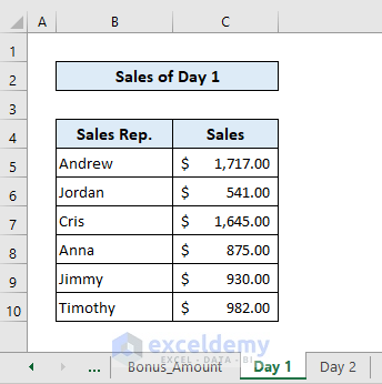
The following worksheet is the sales data for Day 1 in November 2021.
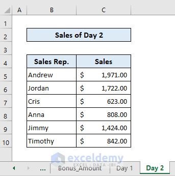
The worksheet with the name ‘Day 2’ is here with the sales data for the second day.
- Here’s what you need to insert in Cell C5 in the Bonus_Amount worksheet:
=VLOOKUP(SUMPRODUCT(SUMIF(INDIRECT("'"&$H$5:$H$6&"'!"&"B5:B10"),Bonus_Amount!B5,INDIRECT("'"&$H$5:$H$6&"'!"&"C5:C10"))),$E$5:$F$8,2,TRUE)
- Press Enter and use the Fill Handle to autofill the rest of the cells in the Bonus column.
How Does the Formula Work?
- In this formula, the INDIRECT function refers to the Sheet names from Cells H5 and H6.
- The SUMIF function uses the reference sheets (Obtained by the INDIRECT function) to include the sum range and criteria for its arguments. The resultant outputs from this function return an array that represents the sales amounts for a specific salesperson from Day 1 and Day 2.
- The SUMPRODUCT function adds up the sales amounts found in the previous step.
- The VLOOKUP function looks for the range of this total sales amount in the table (E4:F8) of Bonus Criteria in the Bonus_Amount sheet. And finally, it returns the bonus amount based on the criteria range for a salesperson.
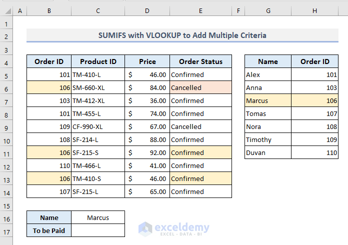
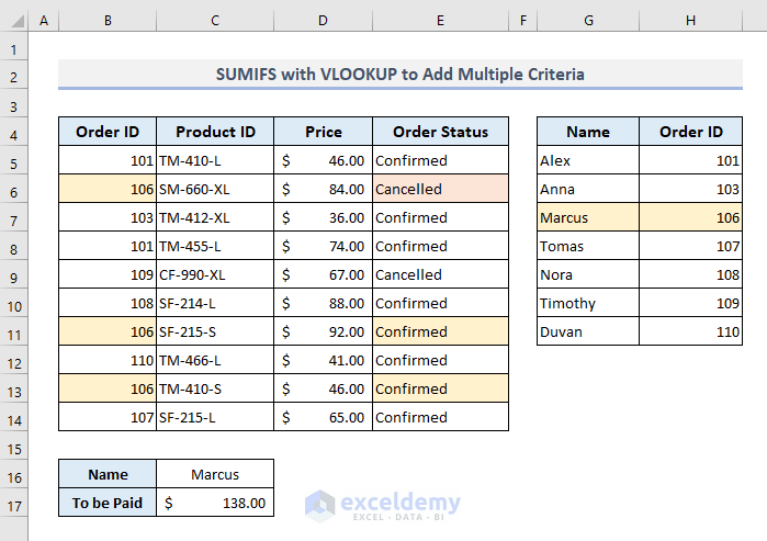
How to Use SUMIFS with VLOOKUP to Add Multiple Criteria in Excel
In this table, we’ve added a new column after the Price column. The new column represents the order statuses for all order IDs. By using the SUMIFS function here, we’ll insert two criteria: the specific order ID for a customer, and the Order Status as ‘Confirmed’ only.
- The required formula in the output Cell C17 will be:
=SUMIFS(D5:D14,B5:B14,VLOOKUP(C16,G5:H11,2,FALSE),E5:E14,"Confirmed")
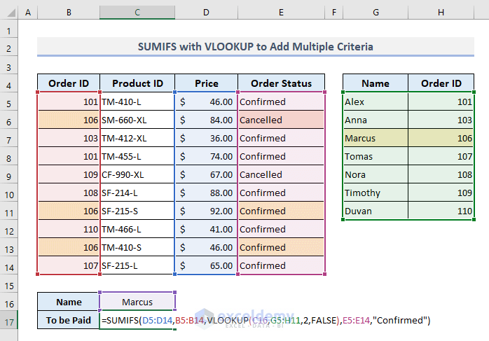
Press Enter, and you’ll get the total price of the conformed orders for the text provided in the Name cell.
Read more: How to Use IF ISNA Function with VLOOKUP in Excel
Download the Practice Workbook
Related Articles
- Combining SUMPRODUCT and VLOOKUP Functions in Excel
- How to Use VLOOKUP with COUNTIF
- INDEX MATCH vs VLOOKUP Function
- Excel LOOKUP vs VLOOKUP
- XLOOKUP vs VLOOKUP in Excel
- How to Use Nested VLOOKUP in Excel
- IF and VLOOKUP Nested Function in Excel
- How to Use VLOOKUP Function with INDIRECT Function in Excel
- How to Use IFERROR with VLOOKUP in Excel
- VLOOKUP with IF Condition in Excel
- Use VLOOKUP to Sum Multiple Rows in Excel
<< Go Back to Excel VLOOKUP Sum | Excel VLOOKUP Function | Excel Functions | Learn Excel
Get FREE Advanced Excel Exercises with Solutions!
