How to Go to Last Non Empty Cell in Column in Excel (9 Easy Ways)

Users often need to find the last non-empty cell of a column. In a long dataset, it is quite time-consuming to find the last non-empty cell or the value of that cell. In this article, we will discuss 9 ways how to go to the last non-empty cell in a column in Excel.

How to Go to Last Non Empty Cell in Column in Excel (9 Handy Ways)

In this article, we will learn 9 ways to go to the last non-empty cell in Excel. Firstly, we will use the XMATCH function. Secondly, we will go for the XLOOKUP function. Thirdly, we will utilize a keyboard shortcut. Then, we will use a combination of the SUMPRODUCT, MAX, and ROW functions. After that, we will combine the INDEX, MAX, and ROW functions. Afterward, we will apply the OFFSET and COUNTA functions together. Next, we will use the INDEX and COUNTA functions in conjunction to get the result. In the penultimate method, we will opt for the LOOKUP function to do our job. Finally, we will resort to a VBA code to go to the last non-empty cell in a column in Excel.

1. Using XMATCH Function

The XMATCH function locates a specified item within an array or cell range and then returns the item’s position within the array or range. In this method, we will use this feature of the function to get the position of the last non-empty cell in a column in Excel.

Steps:

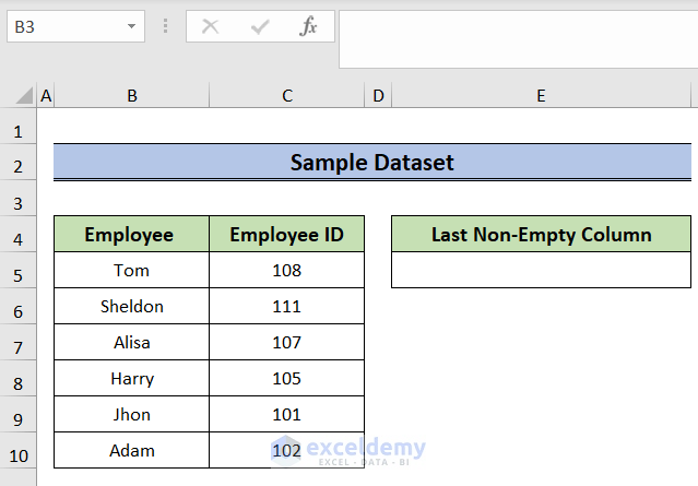
Firstly, select the E5 cell and write the following formula:

=XMATCH("*",B:B,2,-1)

Then, hit Enter.

Consequently, we will find the row number of the last nonempty cell of the column.

Here, the first argument of the function, “*”, denotes what to look for in the column. The asterisk sign means it will look for cells with values. The next argument, B:B, indicates the range of cells the function will look for values. The next argument, 2, denotes a Wildcard character match. This match is employed when the exact content of the cell is not known. Finally, the -1 means it will match from bottom to top. Thus, it will find the last nonempty value in the dataset

2. Applying XLOOKUP Function

To find items in a table or range by row, we use the XLOOKUP function. In this method, we will use this Excel function to find the value of the last non-empty cell of a column.

Steps:

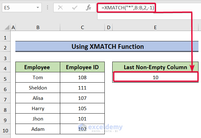
To begin with, select the E5 cell and write the following formula:

=XLOOKUP("*",B:B,B:B,"",2,-1)

Then, press Enter.

As a result, the function will return the content of the last nonempty cell in the column.

Here, the first argument is a Wildcard character. It is used when we do not know the content of a cell. The next argument is the look_array. In this case, it is B:B. The third argument is the return_array. It is also B:B, as we will return the value from the same array. The next argument is a blank character. If the function finds no match, it will return the blank character. The following argument, 2, stands for Wildcard character match. When the exact contents of the cell are unknown, this match is used. The final -1 indicates that the order will match from bottom to top. Thus, it will find the last nonempty value in the dataset.

3. Using Keyboard Shortcut

In this instance, we will use a keyboard shortcut Ctrl+Down Arrow to go to the last nonempty cell of a column.

Steps:

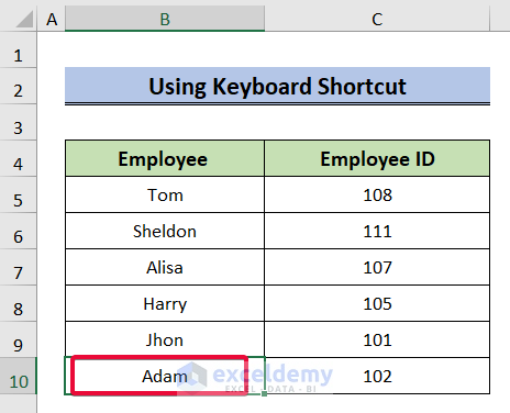
Firstly, select the first cell of the column.
In this case, we will select the B5
Then, hit Ctrl+Down Arrow.

Consequently, we will reach the last nonempty cell.

Note:

This method is applicable only when there is no empty row in between the datasets.

4. Combining SUMPRODUCT, MAX, and ROW Functions

The SUMPRODUCT function returns the sum of the products of the ranges or arrays that are given as an argument of the function. In this method, we will combine it with the MAX and ROW functions to get the position of the last non-empty cell in a column in Excel.

Steps:

To start with, select the E5 cell and write the formula below,

=SUMPRODUCT(MAX(($B:$B<>"")*(ROW(B:B))))

Then, hit Enter.

As a result, we will get the row number of the last nonempty cell.

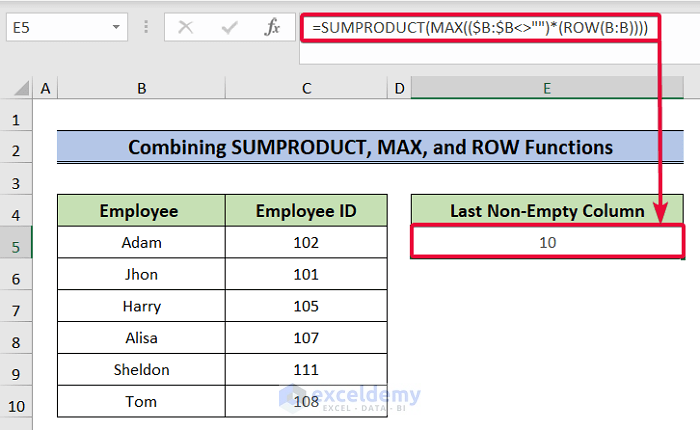
🔎 Formula Breakdown:

ROW(B:B): The ROW function returns the row number of all the cells in the B column.
MAX(($B:$B<>””)*(ROW(B:B))): The MAX function returns the maximum value in an array. Here, the “$B:$B<>””” is a condition. This condition validates if the cells in the range are nonempty or empty and create an array of TRUE and FALSE. If empty,it assigns FALSE; if not, it assigns TRUE. Then, this array gets multiplied with the array returned by the ROW function. Finally, the MAX function returns the row of the cell that has the maximum value in the array of the ROW function. In this case, it is 10.
SUMPRODUCT(MAX(($B:$B<>””)*(ROW(B:B)))): Finally, the SUMPRODUCT returns the product of the MAX array with the ROW array which is 10.

5. Using Combination of INDEX, MAX, and ROW Functions

The INDEX function extracts a value from a table or range, or a reference to a value, and returns it. In this example, we will combine the INDEX, MAX, and ROW functions to get the value of the last cell in a column.

Steps:

To start with, write the following formula after selecting the E5 cell,

=INDEX(B:B,INDEX(MAX(($B:$B<>"")*(ROW(B:B))),0))

Then, hit the Enter key.

As a result, the value of the last nonempty cell will be on the screen.

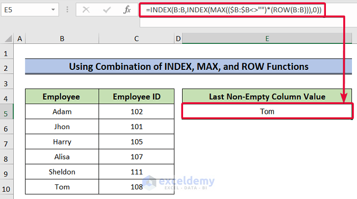
🔎 Formula Breakdown:

(ROW(B:B): The ROW function returns the row number of all the cells in the B column.
MAX(($B:$B<>””)*(ROW(B:B))): The MAX function returns the maximum value in an array. Here, the “$B:$B<>””” is a condition. This condition validates if the cells in the range are nonempty or empty and create an array of TRUE and FALSE. If empty,it assigns FALSE; if not, it assigns TRUE. Then, this array gets multiplied with the array returned by the ROW function. Finally, the MAX function returns the row of the cell that has the maximum value in the array of the ROW function. In this case, it is 10.
INDEX(B:B,INDEX(MAX(($B:$B<>””)*(ROW(B:B))),0)): Finally, the INDEX function in the parenthesis returns the product of the MAX array and the ROW array, which is 10. This means the value 10 refers to the 10th cell in the reference range B:B of the INDEX function outside the parenthesis. So the INDEX function returns the value in the 10th cell, which is “Tom”.

6. Applying OFFSET and COUNTA Functions Together

The OFFSET function returns a reference to a range that is separated from a cell or a range of cells by a specified number of rows and columns. The COUNTA function returns the number of cells that are not empty. Here, we will combine these to get the value of the last non-empty cell in a column.

Steps:

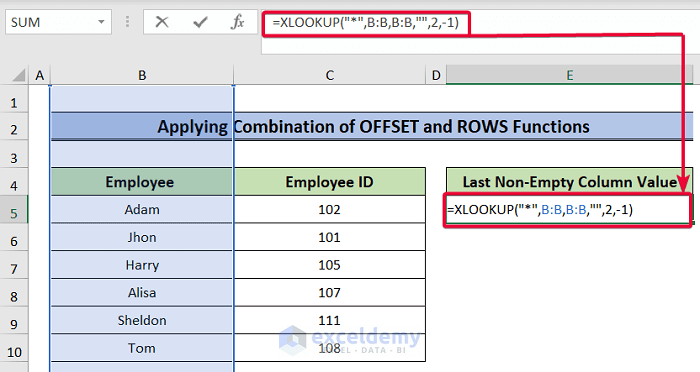
First, select the E5 cell and write the following formula down,

=OFFSET(B4,COUNTA(B4:B10)-1,0)

Then, press the Enter button.

Consequently, we will get the value of the last nonempty cell in the E5 cell.

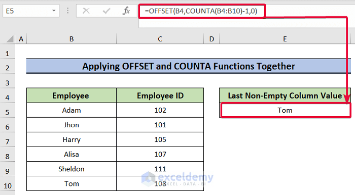
🔎 Formula Breakdown:

COUNTA(B4:B10): The COUNTA function counts the number of non-empty cells in a given range. In this case, the number of nonempty cells in the B4:B10 range is 7.
OFFSET(B4,COUNTA(B4:B10)-1,0): The OFFSET function takes the B4 cell as a reference. The function’s next two arguments- rows and cols– respectively, define how many rows and columns to move from the reference cell. Here, the rows argument is COUNTA(B4:B10)-1 or 7-1 or 6. The cols argument is That means the OFFSET function will return the value of the cell that is 6 cells below the B4 cell. In this case, the value is “Tom”.

7. Combining INDEX and COUNTA Functions

With the help of the INDEX function, you can retrieve a value from a table, a range, or a reference to a value. In this instance, we will use this function together with the COUNTA function.

Steps:

Initially, choose cell E5 and enter the following formula:

=INDEX(B4:B10,COUNTA(B4:B10),0)

Then, hit Enter.

We will therefore obtain the value of the final nonempty cell in the E5 cell.

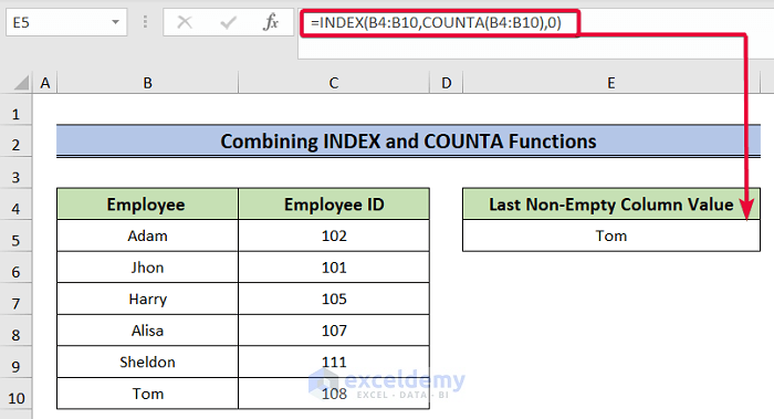
🔎 Formula Breakdown:

COUNTA(B4:B10): The COUNTA function counts the number of non-empty cells in a given range. In this case, the number of nonempty cells in the B4:B10 range is 7.
INDEX(B4:B10,COUNTA(B4:B10),0): The INDEX function numbers the cells of the range that is given as a reference. Here, the INDEX function will number the cells in the range B4:B10 from 1 to 7. It will return the value of the cell in the number 7 The value is “Tom”.

8. Using LOOKUP Function

In this method, we will use the LOOKUP function to go and find the value of the last nonempty cell in a column. The LOOKUP function searches for a reference indicated in the argument and returns the value of the reference cell.

Steps:

At the start, select the E5 cell and type the following formula in the cell,

=LOOKUP(2,1/(B:B<>""),B:B)

Then, hit Enter.

Consequently, we will get the value of the last nonempty cell.

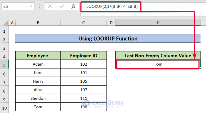
Here, the LOOKUP function searches through the B:B range as indicated by the third argument. It searches if the cells are empty or not through the expression “ B:B<>”” ”.When it assigns TRUE if the cell is non-empty and FALSE otherwise. It returns the result as an array of TRUE and FALSE. Then, it turns the TRUE and FALSE into 1 and -1 respectively. Finally, in the “1/(B:B<>””)” expression, the 1’s and -1’s in the array divide the 1 value and return an array of 1’s and -1’s.Then, the INDEX function looks for 2 in the B:B range. Since the column contains only text data, it can’t find it. So, it returns the largest value in the array that is equal to or less than 2. In this case, it’s the last value in the array, which is “Tom”.

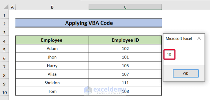
9. Applying VBA Code

In the final method, we will use a simple VBA code to go to the last non-empty cell in a column in Excel.

Steps:

Firstly, select the dataset.
Then, go to the Developer tab in the ribbon.
From there, select the Visual Basic tab.
Consequently, the Visual Basic window will be opened.

After that, in the Visual Basic tab, click on Insert.
Then, select the Module tab.
Consequently, a coding module will appear.

In the coding module, write down the following code.
Then, save the code.

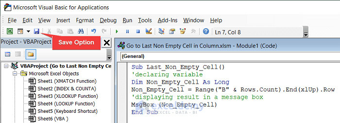
Sub Last_Non_Empty_Cell()
'declaring variable
Dim Non_Empty_Cell As Long
Non_Empty_Cell = Range("B" & Rows.Count).End(xlUp).Row
'displaying result in a message box
MsgBox (Non_Empty_Cell)
End Sub

Then, run the code from the Run tab.

Consequently, we will see the row number of the last nonempty cell in a message box.

Download Practice Workbook

You can download the practice workbook from here.

Go to Last Non Empty Cell in Column.xlsm

Conclusion

In a long Excel dataset, it takes a significant amount of time to go to the last non-empty cell in a column. These methods will allow users to go to the last nonempty cell and fetch the value or the row number of the cell in no time in Excel.