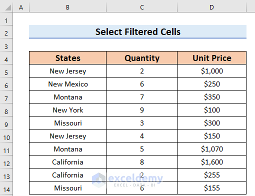
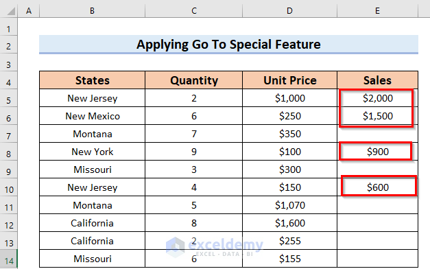
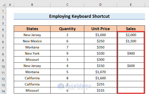
The sample dataset, contains 3 columns, States, Quantity, and Unit Price.
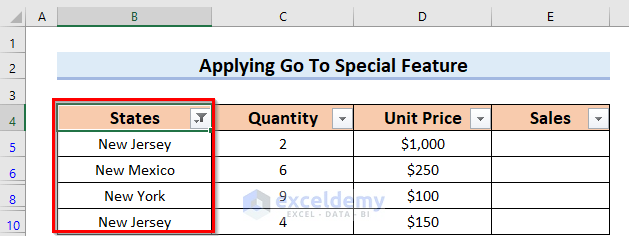
Method 1 – Employing Go To Special feature to Select Only Filtered Cells in Formula
- Select the relevant cells to apply the formula.
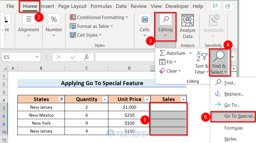
- From the Home tab >> go to Editing >> select Find & Select command >> choose Go To Special option.
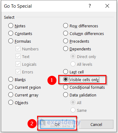
- A dialog box named Go To Special will appear.
- Check Visible cells only.
- Click OK to save the changes.
- Click the Equal (=) key to enter the following formula. Do not click onto anything else as this may unselect the Filtered cells.
=D5*C5In this formula, the Unit Price is multiplied by Quantity to get the Sales amount.
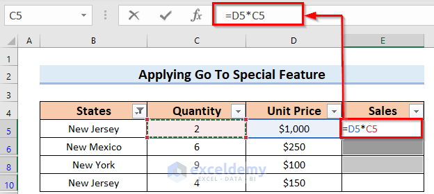
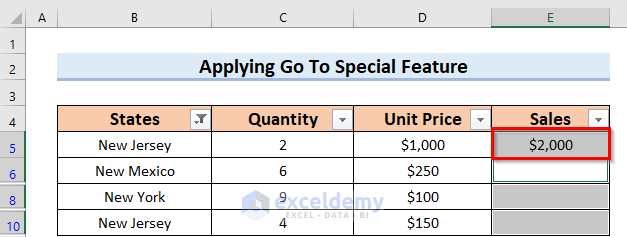
- Press ENTER to get the result.
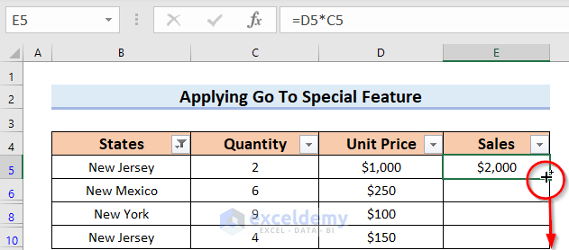
- Drag the Fill Handle icon to fill the other Filtered cells of the column (E6, E8, and E10).
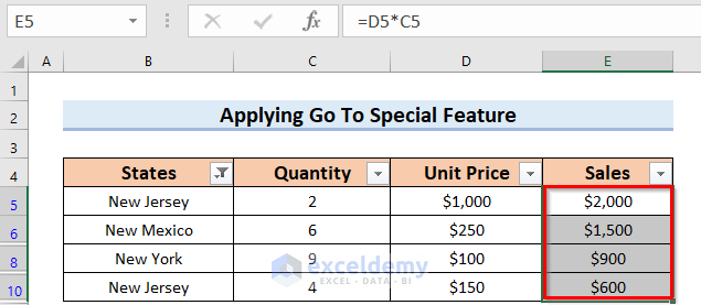
Removing the filter shows that the multiplication formula applied only to the Filtered cells.
Read More: Select All Cells with Data in Excel
Method 2 – Using Keyboard Shortcuts to Select Only Filtered Cells in Excel Formula
Steps:
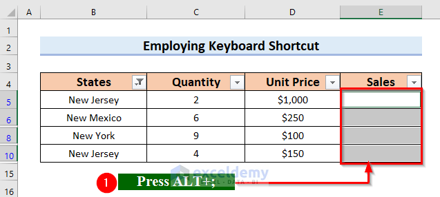
- Select the Filtered cells.
- Press the ALT+; keys to apply the following Excel Formula only in the Filtered Cells.
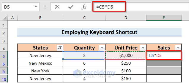
- Click the Equal (=) key to enter the following formula. Do not click onto anything else as this may unselect the Filtered cells.
=C5*D5Quantity is multiplied by Unit Price to get the Sales amount.
- Then, press CTRL+ENTER to get all the Sales amount.
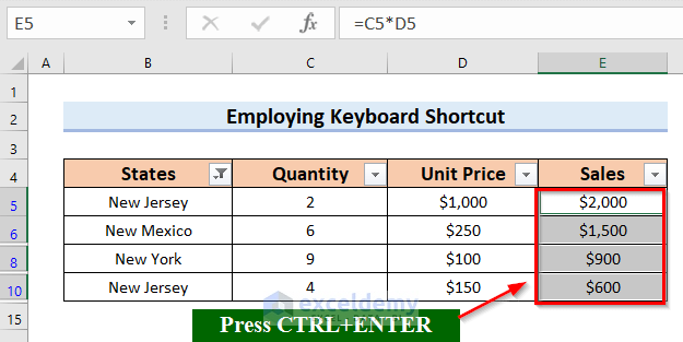
Here, you can see the multiplication formula applied in only the Filtered cells.
Read More: Select All Cells with Data in a Column in Excel
Method 3 – Using the Quick Access Toolbar to Select Only Filtered Cells
Steps:
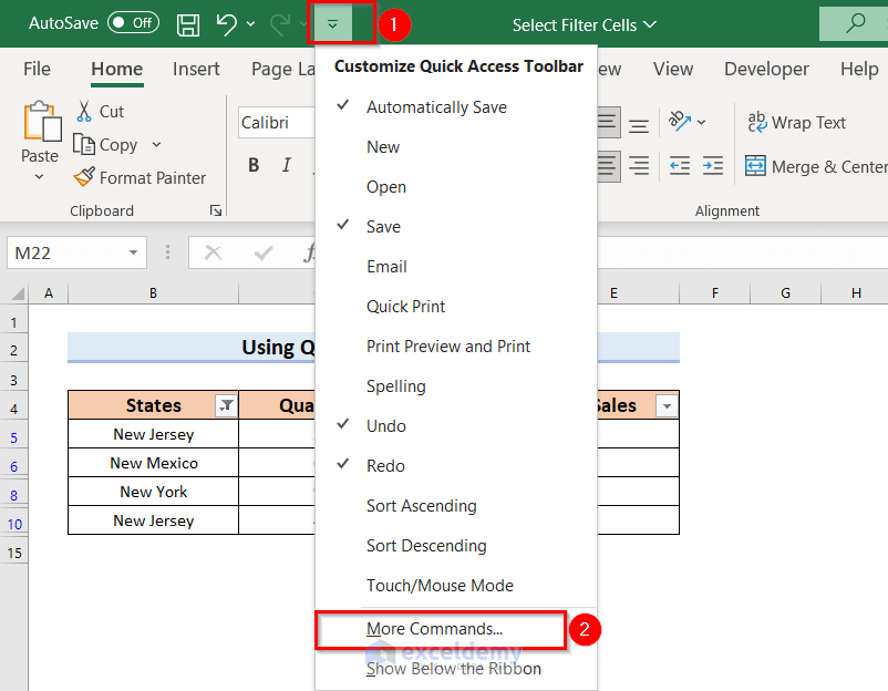
- Click on the Customize Quick Access Toolbar.
- Choose the More Commands option.
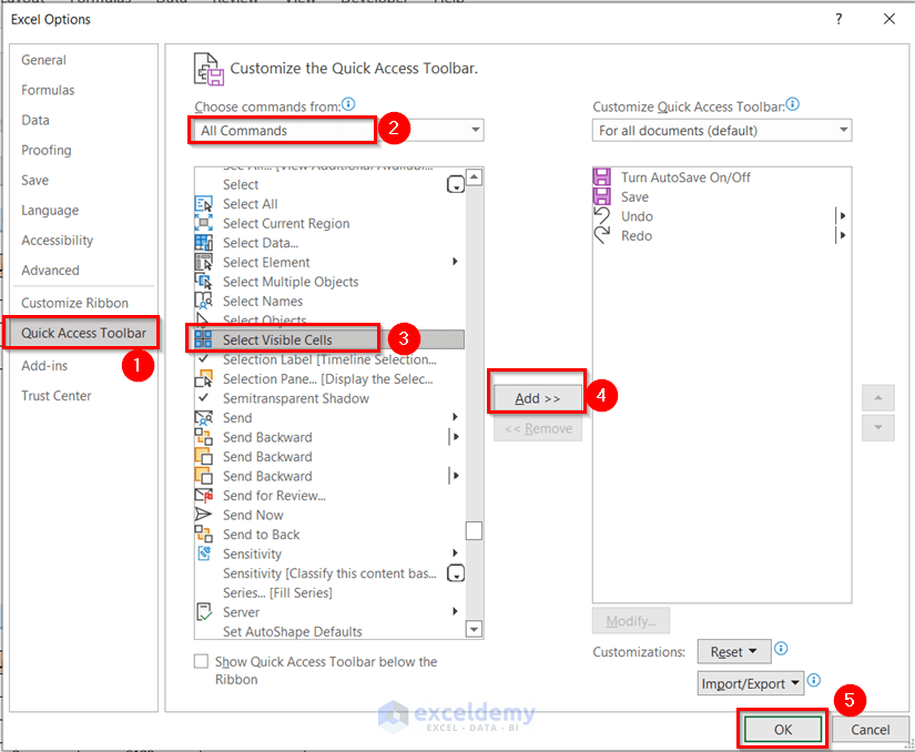
A dialog box named Excel Options will appear.
- Select the Quick Access Toolbar.
- Choose All Commands in the Choose commands from section.
- Choose Select Visible Cells.
- Click on Add >>.
- Click on OK to make the changes.
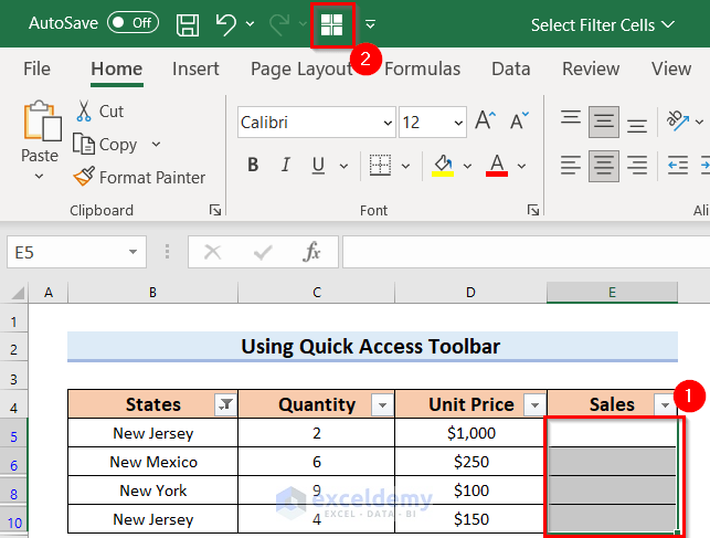
There will now be a new option in the Toolbar named Select Visible Cells.

- Select the Filtered cells.
- Click on the Select Visible Cells Toolbar.
- Click the Equal (=) key to enter the following formula. Do not click onto anything else as this may unselect the Filtered cells.
=C5*D5
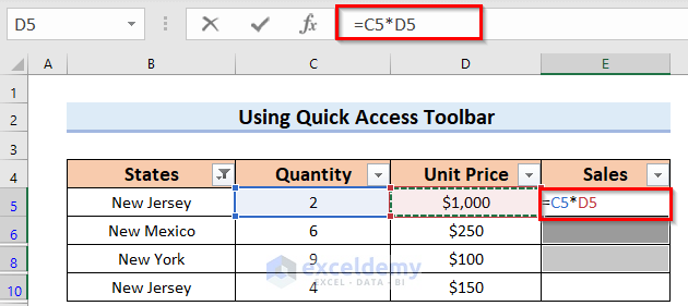
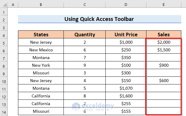
- Press CTRL+ENTER to get all the Sales amount for the filtered cells only.
Read More: How to Select Cells with Certain Value in Excel
Method 4 – Use of SUBTOTAL Function to Select Only Filtered Cells
Steps:
- Select a cell where you want to see the result.
- Enter =SUBTOTAL in that cell.
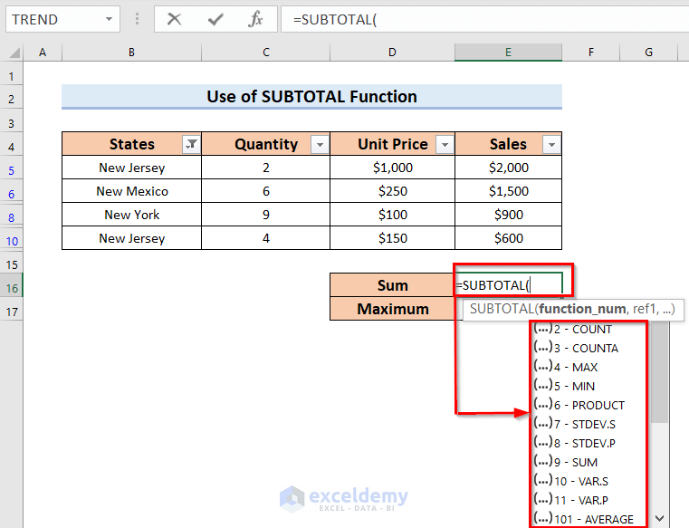
- To find the sum of the Filtered Sales, enter the below formula in cell E16.
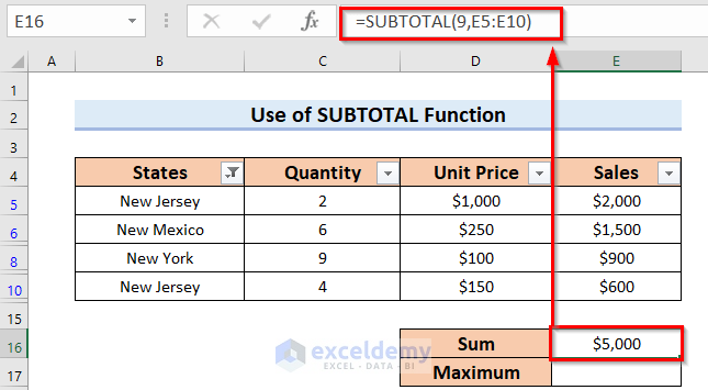
=SUBTOTAL(9,E5:E10)In this formula, 9 denotes the SUM Function. Which will return the summation of the data range E5:E10. But this SUBTOTAL function will only add the visible cell values together.
- Press Enter.
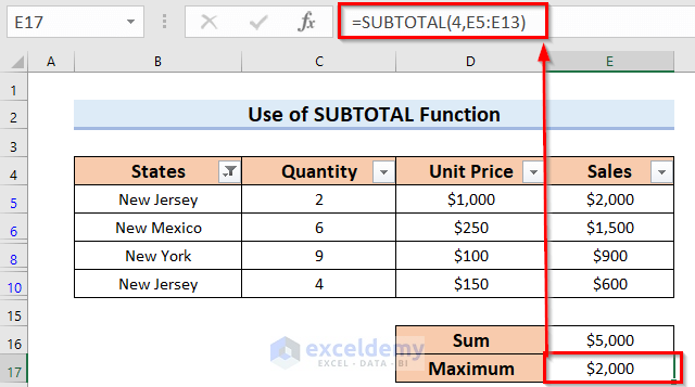
The Subtotal formula includes a number of other functions such as the MAX Function.
- To use this enter the following formula in cell E17.
=SUBTOTAL(4,E5:E10)In this formula, 4 denotes the MAX function. This will return the maximum value of the data range E5:E10 only for the visible cell values.
- Press Enter.
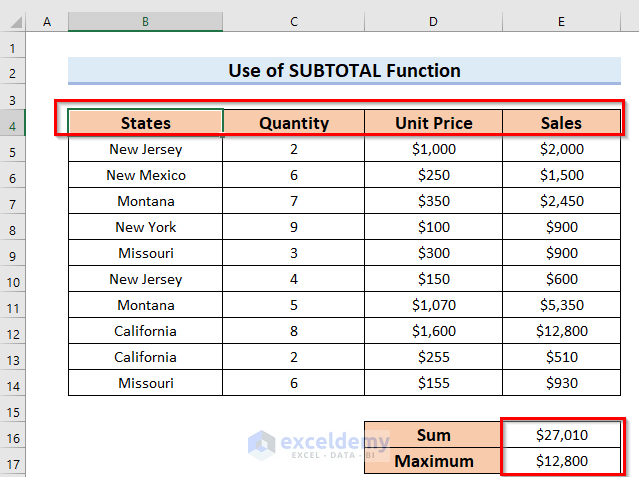
If you unfilter the cells then those formulas will be applicable for all the cells.
Read More: How to Select Random Cells in Excel
Method 5 – Applying AGGREGATE Function to Select Only Filtered Cells
Steps:
- Select a cell where you want to see the result.
- Enter =AGGREGATE.
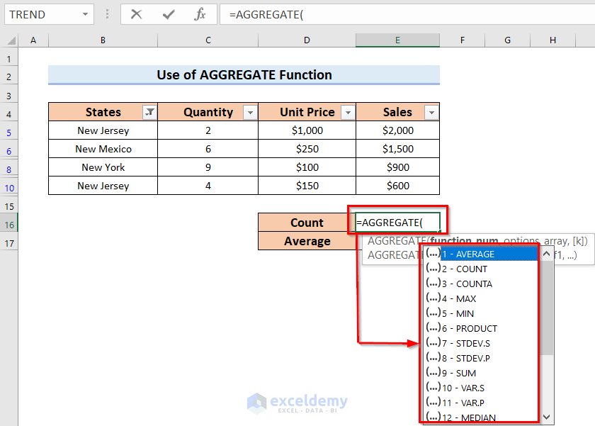
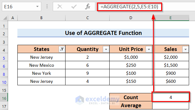
- To apply the formula to the Filtered cells only, choose option 5 – Ignore hidden rows.
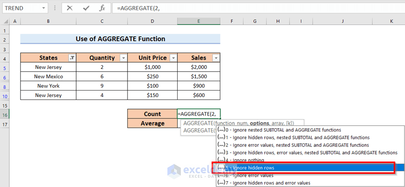
- Enter the below formula in cell E16.
=AGGREGATE(2,5,E5:E10)In this formula, 2 denotes the COUNT function. Which will return the total cell count of the data range E5:E10, while 5 denotes that this function will ignore the hidden rows.
- Press Enter.
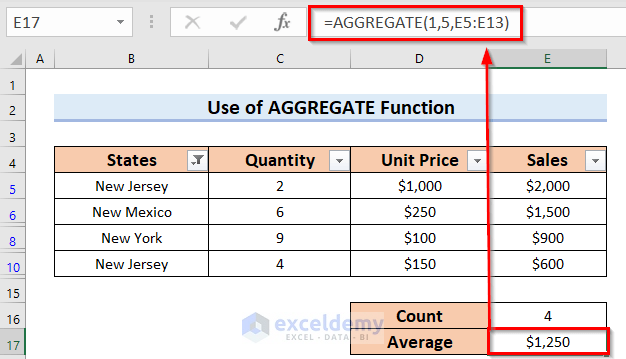
The AGGREGATE function also includes the AVERAGE function.
- Enter the below formula in cell E17.
=AGGREGATE(1,5,E5:E10)In this formula, 1 denotes the AVERAGE function, which will return the average of the data range E5:E10, while 5 denotes that the AVERAGE function will ignore only the hidden rows.
- Press Enter.
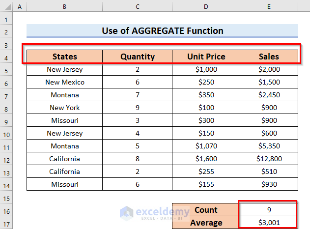
If you unfilter the cells then those formulas will be applicable for all the cells.
Read More: How to Select Blank Cells in Excel and Delete
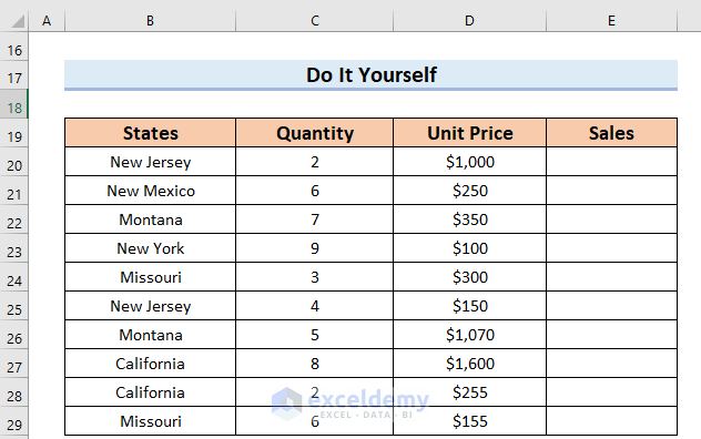
Practice Section
Download Practice Workbook
You can download the practice workbook from here:
Related Articles
- How to Select Highlighted Cells in Excel
- [Fixed!] Selected Cells Not Highlighted in Excel
- Selecting Non-Adjacent or Non-Contiguous Cells in Excel
<< Go Back to Select Cells | Excel Cells | Learn Excel
Get FREE Advanced Excel Exercises with Solutions!
