Consider a dataset of Salesmen of an organization and their respective Sales over a certain period of time. We want to select some random cells from this list.
Method 1 – Combining RAND, INDEX, and RANK.EQ Functions to Select Random Cells in Excel
Steps:
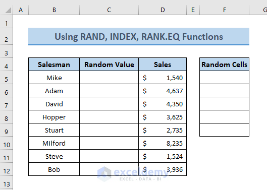
- Create two new columns with the headings Random Value and Random Cells.
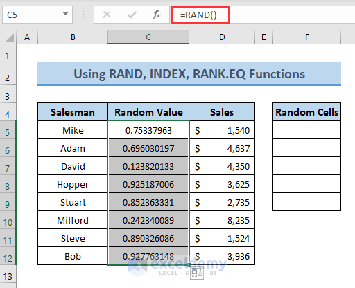
- Use the following formula in the first cell under the Random Value column.
=RAND()
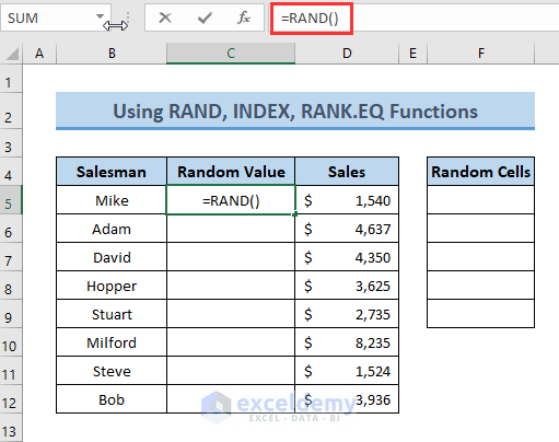
- Press Enter, and the cell will show a random value for the function.
- Drag the Fill Handle tool down the column.
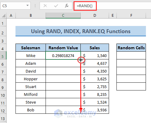
- Excel will Autofill the formula.
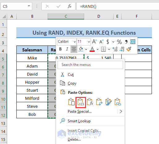
- Copy the cells and use the Paste Special option (i.e. Paste Values) to paste the values only.
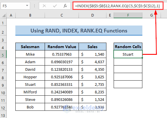
- Apply the following formula to the first cell under the Random Cells column to show a randomly selected cell.
=INDEX($B$5:$B$12,RANK.EQ(C5,$C$5:$C$12),1)
- $B$5:$B$12= Range of the Salesman
- $C$5:$C$12= Range of the Random Value
- C5= Random value
Formula Breakdown
RANK.EQ(C5,$C$5:$C$12) gives the rank of the cell value of C5 (i.e. 0.75337963) in the range $C$5:$C$12. So, it returns 5.
INDEX($B$5:$B$12,RANK.EQ(C5,$C$5:$C$12),1) returns the value at the intersection of Row 5 and Column 1. So, the output is Stuart.
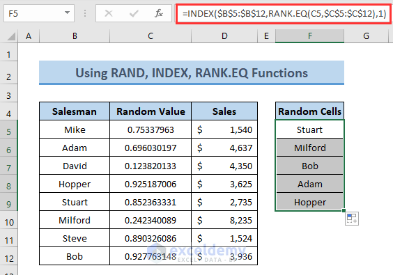
- Drag the formula down and you will be able to select the random cells.
Read More: Select All Cells with Data in Excel
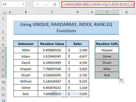
Method 2 – Selecting Random Cells with UNIQUE, RANDARRAY, INDEX, and RANK.EQ Functions
Steps:
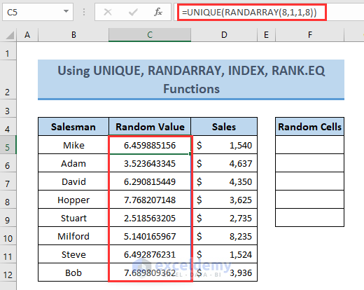
- Use the following formula to get a random value.
=UNIQUE(RANDARRAY(8,1,1,8)
Here,
- 8= Total number of Rows
- 1= Total number of Columns
- 1= Minimum number
- 8= Maximum number
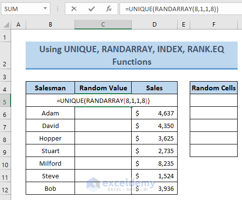
- Press Enter, and all the cells will show corresponding random values for the Salesman Column.
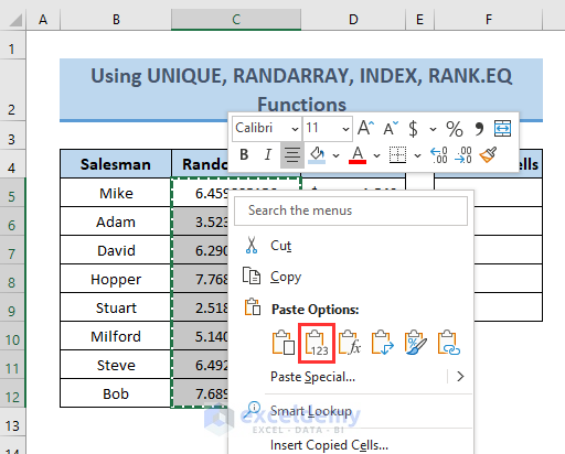
- Copy the cells and paste the values only to convert the formulas into values.
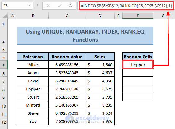
- Apply the following formula to get the randomly selected cell:
=INDEX($B$5:$B$12,RANK.EQ(C5,$C$5:$C$12),1)
Here,
- $B$5:$B$12= Range of the Salesman
- $C$5:$C$12= Range of the Random Value
- C5= Random value
Formula Breakdown
RANK.EQ(C5,$C$5:$C$12) gives the rank of the cell value of C5 (i.e. 0.75337963) in the range $C$5:$C$12. So, it returns 4.
INDEX($B$5:$B$12,RANK.EQ(C5,$C$5:$C$12),1) returns the value at the intersection of Row 4 and Column 1. So, the output is Hopper.
- Drag the formula down to get the random cells.
Read More: Select All Cells with Data in a Column in Excel
Method 3 – Applying RAND, INDEX, RANK.EQ, and COUNTIF Functions
Steps:
- Follow Method 1 to get the Random Values with the RAND function.
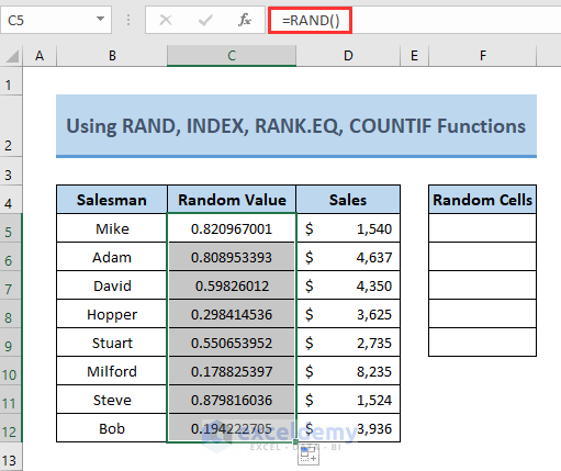
- Apply the following formula to get a randomly selected cell.
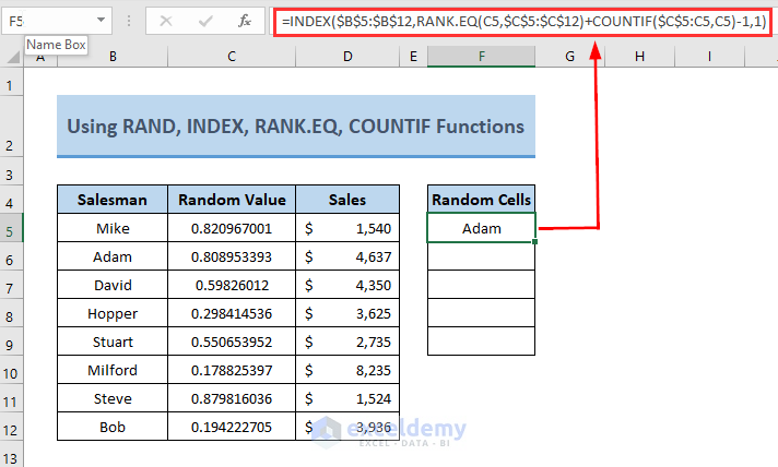
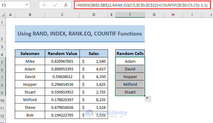
=INDEX($B$5:$B$12,RANK.EQ(C5,$C$5:$C$12)+COUNTIF($C$5:C5,C5)-1,1)
Here,
- $B$5:$B$12= Range of the Salesman
- $C$5:$C$12= Range of the Random Value
- C5= Random value
Formula Breakdown
RANK.EQ(C5,$C$5:$C$12) gives the rank of the cell value of C5 (i.e. 0.75337963) in the range $C$5:$C$12. So, it returns 2.
COUNTIF($C$5:C5,C5) returns the number of cells with the value of C5. So, it gives 1.
2+1-1=2
INDEX($B$5:$B$12,RANK.EQ(C5,$C$5:$C$12)+COUNTIF($C$5:C5,C5)-1,1) returns the value at the intersection of Row 2 and Column 1. So, the output is Adam.
- Drag the formula to the next cells to get the output.
Read More: How to Select Cells with Certain Value in Excel
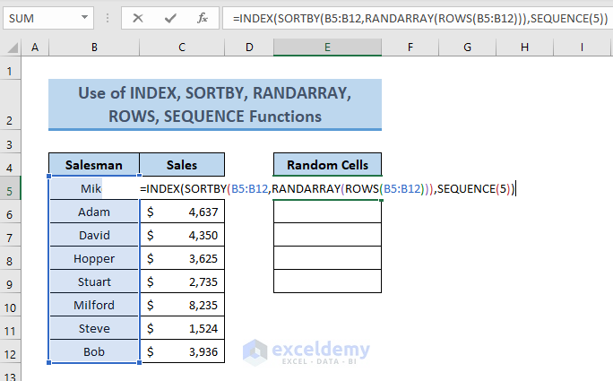
Method 4 – Use INDEX, SORTBY, RANDARRAY, ROWS, and SEQUENCE Functions to Choose Random Cells
Steps:
- Use the following formula to get a selected cell.
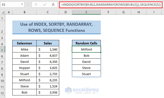
=INDEX(SORTBY(B5:B12,RANDARRAY(ROWS(B5:B12))),SEQUENCE(5))
Here,
- B5:B12= Range of the Salesman
Formula Breakdown
ROWS(B5:B12) gives the number of rows in the mentioned range= 8.
RANDARRAY(ROWS(B5:B12)) results in random 9 numbers.\
SEQUENCE(5) returns a range of the serial numbers (1 to 5).
Finally, INDEX(SORTBY(B5:B12,RANDARRAY(ROWS(B5:B12))),SEQUENCE(5)) returns 5 cell values.
- Press Enter and you will get the output for all cells you want (i.e. 5).
Read More: How to Select Blank Cells in Excel and Delete
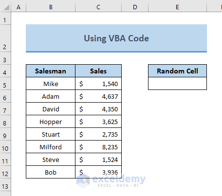
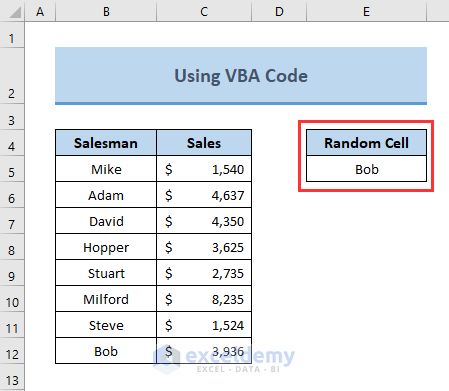
Method 5 – Select Random Cells Using Excel VBA Code
For the same set of data, we will now select a random cell from the given list using a VBA code. The newly created cell (i.e. E5) under the Random Cell column will return the selected random cell.
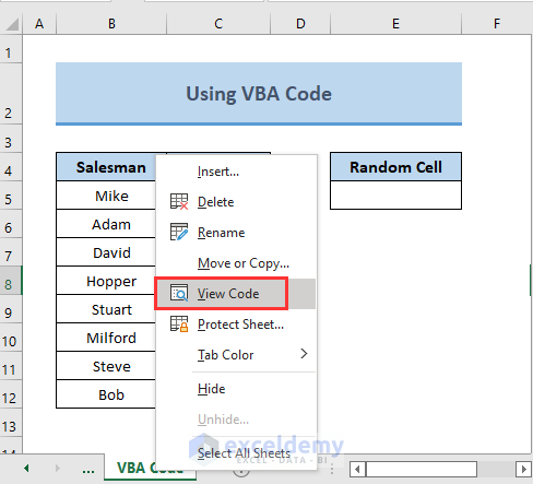
Steps:
- Right-click on the sheet name and select View Code from the options.
- A window for entering the code will appear here.
- Enter the following Code:
Code:
Sub Select1Random_Name()
Dim xCell As Long
xCell = [RandBetween(5,12)]
Cells(5, 5) = Cells(xCell, 2)
End Sub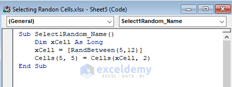
- The output will be shown at cell(5,5) which means cell E5.
Read More: How to Select Highlighted Cells in Excel
Download the Practice Workbook
Related Articles
- How to Select Only Filtered Cells in Excel Formula
- [Fixed!] Selected Cells Not Highlighted in Excel
- Selecting Non-Adjacent or Non-Contiguous Cells in Excel
<< Go Back to Select Cells | Excel Cells | Learn Excel
Get FREE Advanced Excel Exercises with Solutions!

Hi,
I am using Method 1 to pick random name from a column. I have multiple sheets in one document. each time I create a new sheet with equation, all the previous sheets random name changes.
Can you advise why?
regards
Hello Mary
Thanks for visiting our blog and sharing your problem. The issue you are facing is due to the RAND function, which generates a new random number every time the worksheet recalculates.
To prevent the problem, copy the random values, then use Paste Special and paste them back as Values. The idea should keep your random names stable.
Regards
ExcelDemy