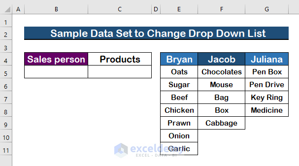
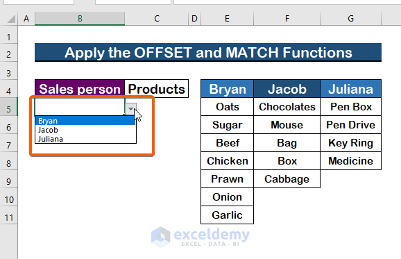
In this tutorial, we will run through the two best ways to change drop-down lists. Firstly, we will apply the OFFSET and MATCH functions in the drop-down lists to make changes based on cell values. Additionally, we will use the XLOOKUP function featured in Microsoft Excel 365 to do the same. In the below image, we have provided a sample data set to accomplish the task.
Method 1 – Combine the OFFSET and MATCH Functions to Change Drop Down List Based on Cell Value in Excel
Step 1: Create a Data Validation List
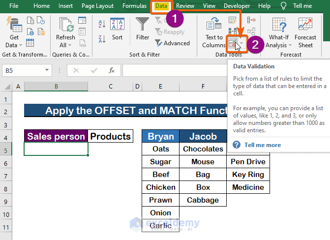
- Go to Data.
- Click on Data Validation.
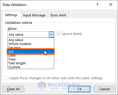
Step 2: Select the source for the List
- From the Allow option, select the List.
- In the source field, select the source range E4:G4 for the names of the salesmen.
- Press Enter.
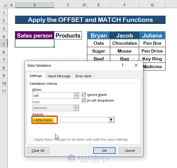
- A drop-down will appear in cell B5.
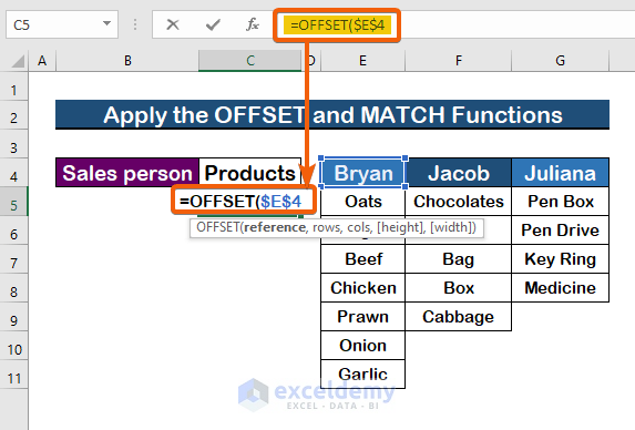
Step 3: Apply the OFFSET function
- Type the following formula for the OFFSET function,
=OFFSET($E$4)- Here, E4 is the reference cell in absolute form.
- In the rows argument, put 1 as the value that will count 1 row down from the reference cell E4.
=OFFSET($E$4,1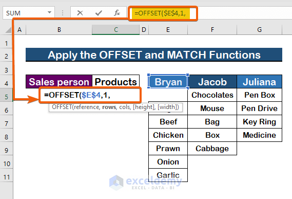
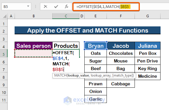
Step 4: Use the MATCH function to define the OFFSET function column
- In the cols argument, to select the columns use the MATCH function with the following formula.
=OFFSET($E$4,1,MATCH($B$5- Here, B5 is the cell value selected in the drop-down list.
- To select the lookup_array argument for the MATCH function, add E4:G4 as the range in absolute form with the following formula.
=OFFSET($E$4,1,MATCH($B$5,$E$4:$G$4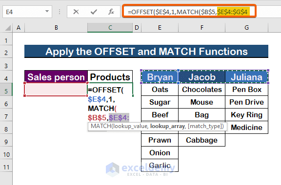
- Type 0 for the Exact match type. The following formula will return 3 for the MATCH
MATCH($B$5,$E$4:$G$4,0)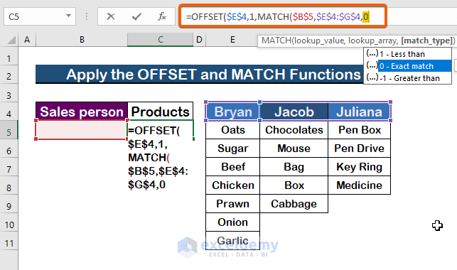
- Write minus 1 (-1) from the MATCH function, because the OFFSET function counts the first column as zero (0).
MATCH($B$5,$E$4:$G$4,0)-1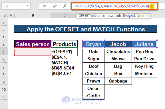
Step 5: Enter the height of the columns
- When selecting 1 in the height argument, it will count that each column has one value.
=OFFSET($E$4,1,MATCH($B$5,$E$4:$G$4,0)-1,1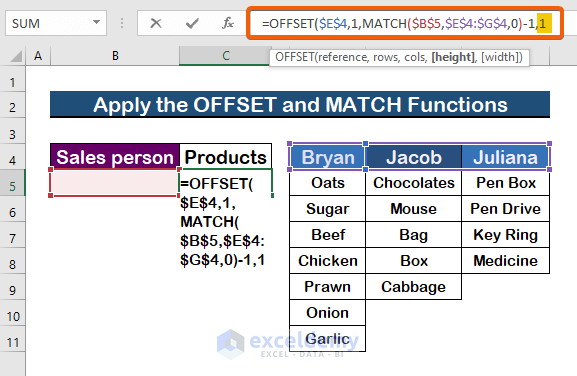
Step 6: Enter the width Value
- For the width argument, type 1.
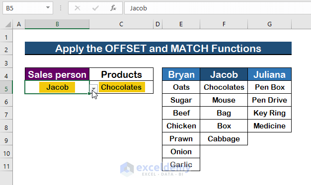
=OFFSET($E$4,1,MATCH($B$5,$E$4:$G$4,0)-1,1,1)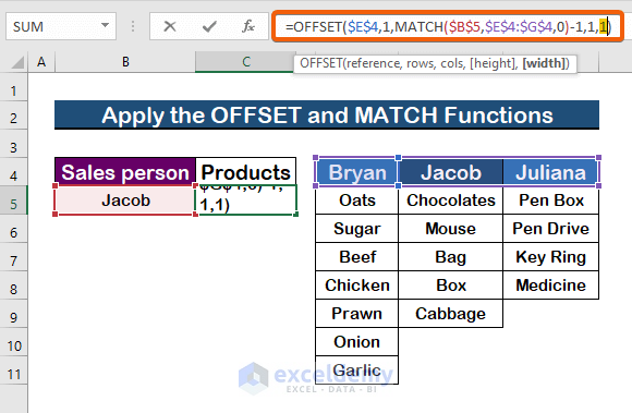
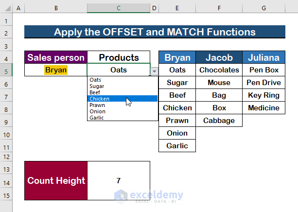
- You will see that when we select Jacob in B5, it will result in Chocolate as the first element for Jacob.
Step 7: Count the elements of each column
- To count the number of elements in a column, we will apply the COUNTA function in cell C13 with the following formula.
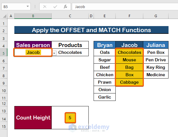
=COUNTA(OFFSET($E$4,1,MATCH($B$5,$E$4:$G$4,0)-1,10))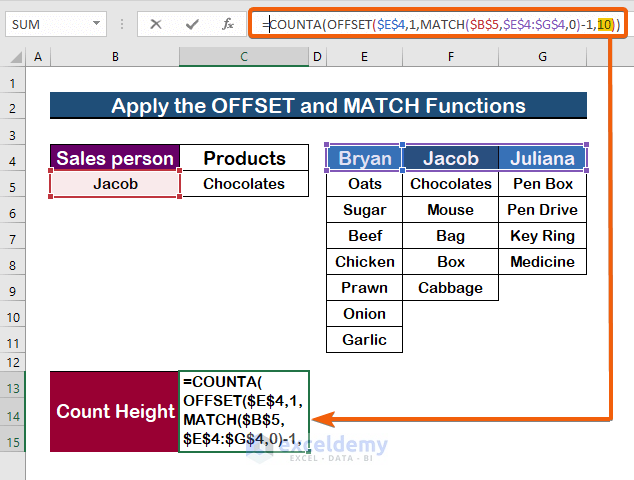
- This will count the element/product number for a particular salesman (Jacob).
Step 8: Enter the count height cell value as the height argument in the OFFSET function
- Write the following formula to add the height.
=OFFSET($E$4,1,MATCH($B$5,$E$4:$G$4,0)-1,C13,1)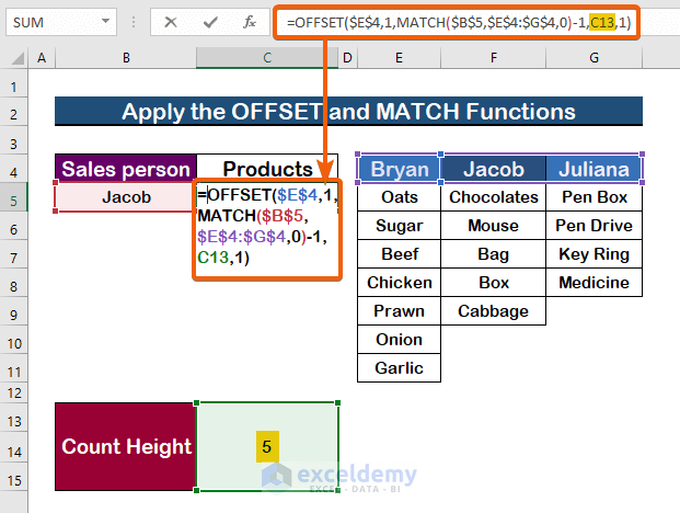
Step 9: Copy the Formula
- Press Ctrl + C to copy the formula.
=OFFSET($E$4,1,MATCH($B$5,$E$4:$G$4,0)-1,C13,1)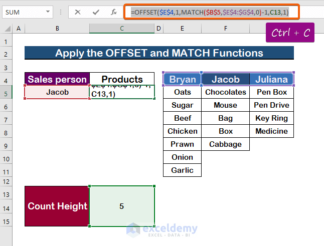
Step 10: Paste the formula
- Paste the formula in the Data Validation source.
=OFFSET($E$4,1,MATCH($B$5,$E$4:$G$4,0)-1,C13,1)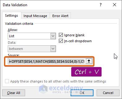
- Press Enter to see the change.
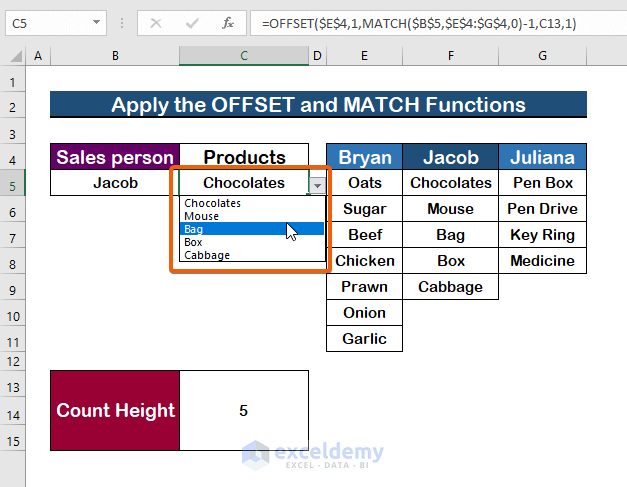
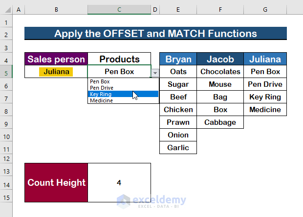
- Your drop-down list values will change based on another cell value.
- Change the cell value Bryan to Juliana and get the product’s name sold by Juliana.
Read More: Create Excel Filter Using Drop-Down List Based on Cell Value
Method 2 – Use the XLOOKUP Function to Change Drop Down List Based On Cell Value in Excel
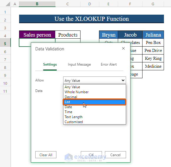
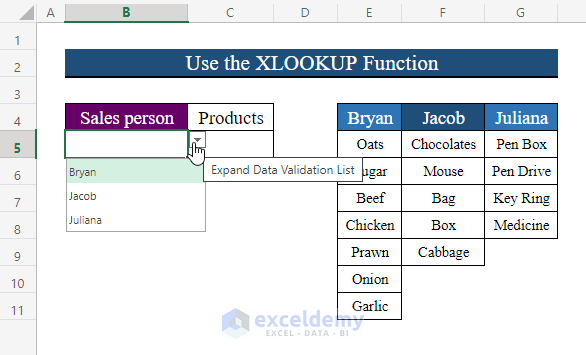
Step 1: Make a Data Validation List
- From the Data Validation option, select the List.
Step 2: Type the source range
- Select the source range E4:G4 in the source box.
- Press Enter.
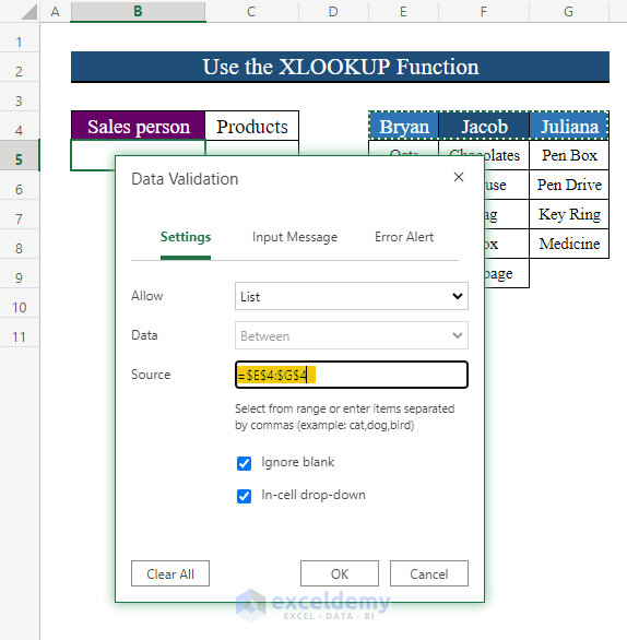
- A Data Validation list will appear.
Step 3: Insert the XLOOKUP function
- Select the B5 cell as the look_up.
=XLOOKUP(B5)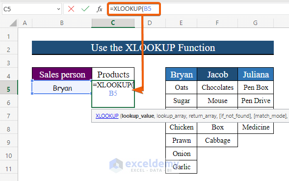
Step 4: Select the lookup array
- Write the range E4:G4 as the lookup_array.
=XLOOKUP(B5, E4:G4)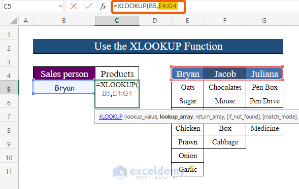
Step 5: Insert the return_array
- Type the range for the return value E5:G11.
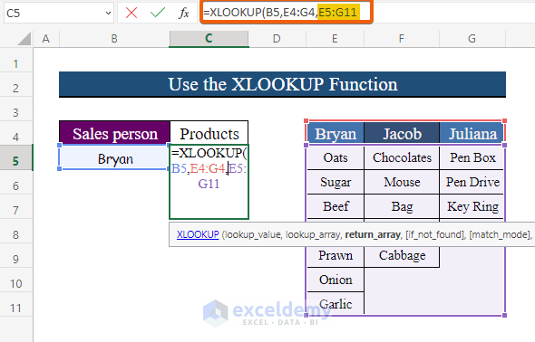
- The products will return according to a particular salesman.
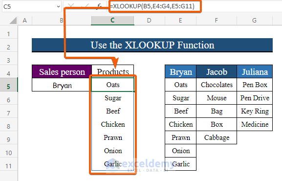
- Select any name from the drop-down list and get the products’ names.
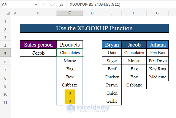
Notes. In the above image, zero is shown as in the range the cells were blank. That’s why these are considered zero. To remove the zeros follow the steps below.
Step 6: Apply the UNIQUE function
- Type the following formula nested with the UNIQUE function.
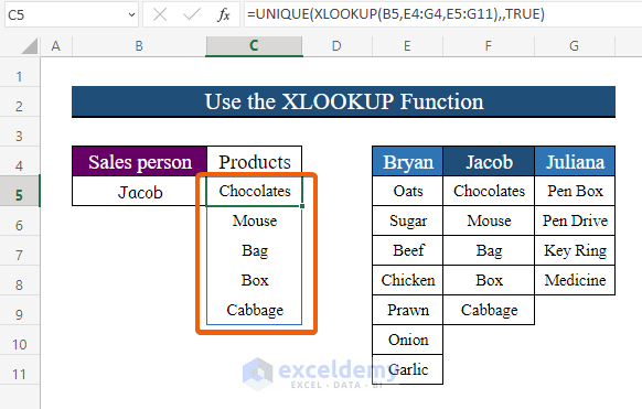
=UNIQUE(XLOOKUP(B5,E4:G4,E5:G11),,TRUE)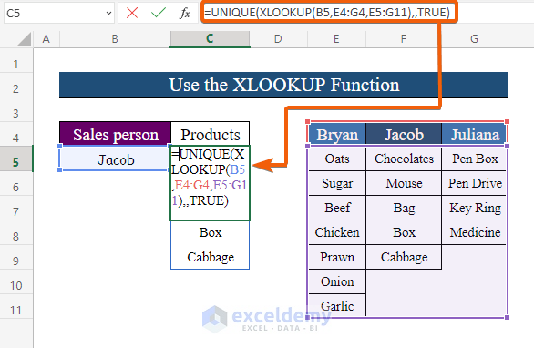
- You will get the result you desired.
Read More: How to Populate List Based on Cell Value in Excel
Download Practice Workbook
Download this practice workbook to exercise while you are reading this article.
Related Articles
- Conditional Drop Down List in Excel
- How to Use IF Statement to Create Drop-Down List in Excel
- How to Create Dynamic Dependent Drop Down List in Excel
- Excel Dependent Drop Down List
- How to Make Dependent Drop Down List with Spaces in Excel
- Excel Formula Based on Drop-Down List
- How to Create Dependent Drop Down List with Multiple Words in Excel
- How to Extract Data Based on a Drop Down List Selection in Excel
<< Go Back to Edit Drop-Down List in Excel | Excel Drop-Down List | Data Validation in Excel | Learn Excel
Get FREE Advanced Excel Exercises with Solutions!

Hello,
That was an amazing guide, more complete and useful than any other instruction that I found on the Internet. Thanks a lot.
Just one question:
For method 2 (Using the Xlookup function) is it possible also to get the final results (list of products) in a row next to each other, other than having them in the same column under each other?
Greetings Sepehr,
Thank you for your appreciation.
# The answer to your question is “Yes“—it is possible to have the list of products in different columns.
# Just use the TRANSPOSE function preceding the UNIQUE+XLOOKUP formula. Of course, you have to have Excel 365 to use the XLOOKUP function.
=TRANSPOSE(UNIQUE(XLOOKUP(B5,B7:D7,B8:D14),,TRUE))