In Microsoft Excel, AND is one of the most frequently used functions and the AND function is applied to check for logical tests under different conditions. In this article, you’ll get to learn how you can use this AND function efficiently with different conditions in Excel.
Here you will also find some articles to use this function with text, return TRUE or FALSE, and Conditional Formatting. AND function can also be used with other functions. You will get some articles to learn how to use this function with other Excel functions in formulas and VBA.
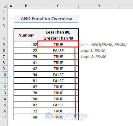
The above screenshot is an overview of the article which represents an application of the AND function in Excel. You’ll learn more about the dataset as well as the methods to use AND function properly in the following sections of this article.
Introduction to the AND Function
- Function Objective:
Checks whether all the arguments are TRUE, and returns TRUE if all arguments are TRUE.
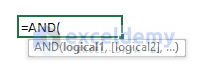
- Syntax:
=AND(logical1, [logical2])
- Arguments Explanation:
| Argument | Compulsory/Optional | Explanation |
|---|---|---|
| logical1 | Compulsory | 1st logical condition. |
| [logical2] | Optional | 2nd logical condition. |
- Return Parameter:
Returns with a logical value- TRUE or FALSE.
How to Use AND Function in Excel: 7 Examples
1. Using AND Function to Test with Logical Values
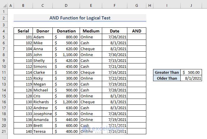
Let’s get introduced to our dataset first that combines a range of data for a charity foundation. Columns C, D, E, and F consist of the donor names, donation amounts, mediums of donations and donation dates respectively. In Column G, by using AND function, we’ll find out the rows where the donors have donated more than $500 before August, 2021.
📌 Steps:
➤ In the output Cell G5, the formula will be:
=AND(D5>$J$11,F5<$J$12)➤ Press Enter and the function will return TRUE that means Adam has donated more than $500 before 1 August, 2021.
➤ Now use Fill Handle to autofill the rest of the cells in Column G.
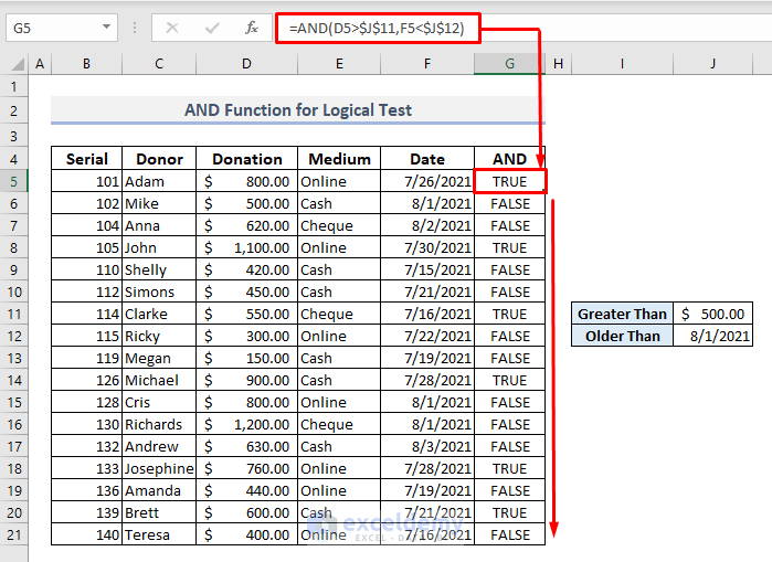
AND function returns with FALSE logical value if any one of the conditions appears FALSE. The function will return TRUE only if all conditions are TRUE.
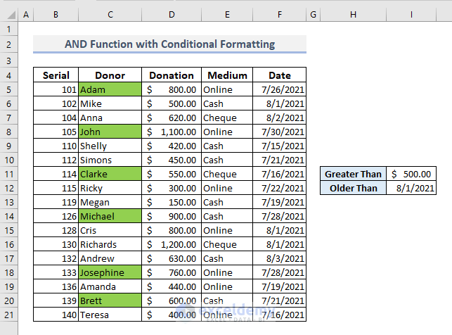
2. Using AND Function with Conditional Formatting
Now we’ll find out the names who have donated more than $500 before 1 August, 2021 by highlighting those names with a color. So, we have to assign a formula and a color in Conditional Formatting for the output data.
📌 Step 1:
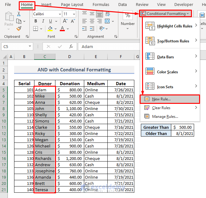
➤ Select all the names in Column C.
➤ Under Home tab, choose New Rule command from the Conditional Formatting drop-down. A dialogue box will open.
📌 Step 2:
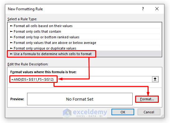
➤ Select “Use a formula to determine which cells to format” as Rule Type,
➤ In the formula box, type:
=AND(D5>$I$11,F5<$I$12)
➤ Press Format and another dialogue box will appear.
📌 Step 3:
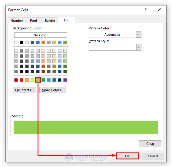
➤ From the Fill option, select a color that you want to see on the output cells in your dataset or table.
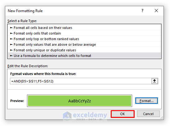
➤ Press OK and a preview will be shown in the New Formatting Rule dialogue box.
📌 Step 4:
➤ Press OK and you’re done.
Like the screenshot below, you’ll find the donor names with the selected color who have donated more than $500 before 1 August, 2021.
Read More: How to Use Conditional Formatting with AND Function in Excel
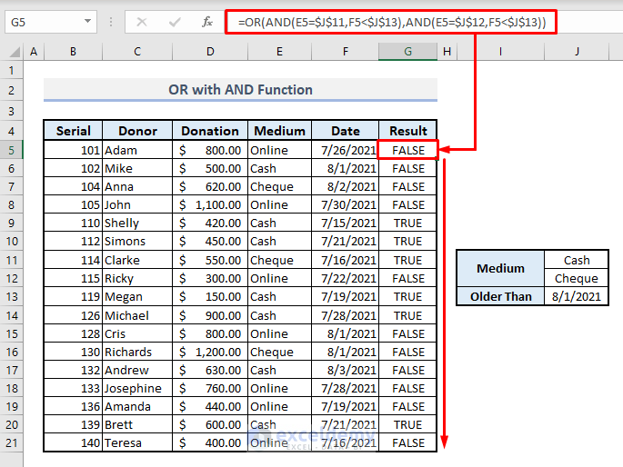
3. Combining OR with AND Function
The OR Function returns with TRUE if any of the conditions found TRUE and returns FALSE if all conditions appear to be FALSE. So, it’s completely opposite to the AND function. By combining OR with AND function, we can add multiple criteria from our dataset. Assuming that we want to find in Column G how many rows contain the donors who have donated through cash or cheque before 1 August, 2021.
📌 Steps:
➤ Select the output Cell G5 and type:
=OR(AND(E5=$J$11,F5<$J$13),AND(E5=$J$12,F5<$J$13))➤ Press Enter, fill down the entire column and you’ll get the results at once.
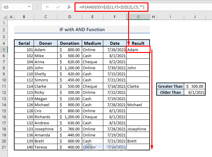
4. Combining IF with AND Function
By using the IF function before AND function, we can add some statements based on the return types of logical values. For example, we want to see the names only in Column G who have donated more than $500 before 1 August, 2021.
📌 Steps:
➤ In the output Cell G5, the related formula will be:
=IF(AND(D5>$J$11,F5<$J$12),C5,"")➤ Press Enter, autofill the entire column and you’re done. You’ll see all the names of the donors based on the selected criteria.
Read More: How to Use IFS and AND Functions Together in Excel
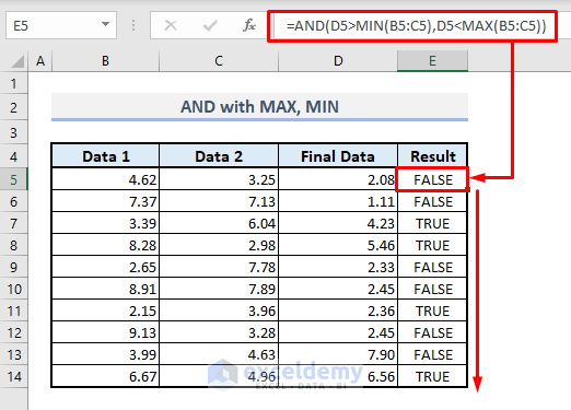
5. Enclosing MIN & MAX Functions with AND
By using MIN and MAX functions inside AND function, we can determine if a value falls between two other values. For example, in our new dataset, Column B and Column C have some experimental results found in a laboratory with iterations. Column D consists of the final results that have to be found between the other two values in the same rows.
📌 Steps:
➤ In Cell E5, the related formula will be:
=AND(D5>MIN(B5:C5),D5<MAX(B5:C5))➤ Press Enter and you’ll find all the return values with TRUE or FALSE. So, if the final data is found between the other two values, then the function will return TRUE, otherwise FALSE.
6. Apply Nested AND Function in Excel
You can check multiple conditions using the nested AND function in Excel. Using the following formula we will check if the donated amount is greater than $300, the medium is Online, and donated after 7/15/2021 and before 8/1/2021.
=AND(D5>$J$10,E5=$J$11,AND(F5<$J$12,F5>$J$13))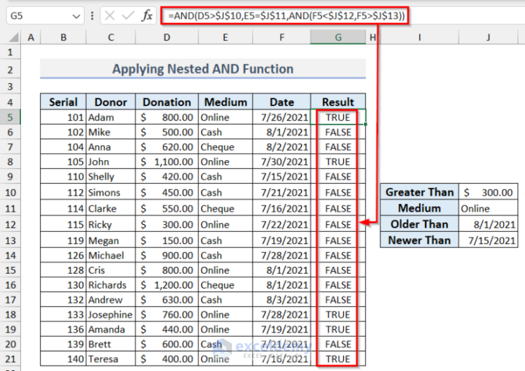
7. Use AND Function with Nested IF Function
You can also use the AND function with the nested IF function in Excel. Here, we will categorize the donors based on the donated amount using the following formula.
=IF(AND(D5>=900),"Major Donor",IF(AND(D5>=500,D5<900),"Regular Donor",IF(AND(D5>0,D5<500),"Small Donor",0)))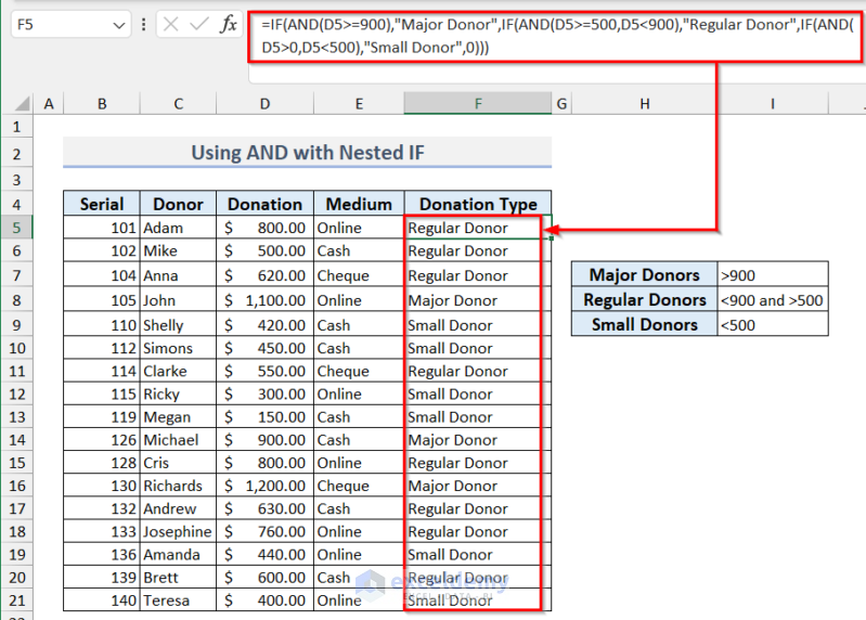
Read More: Nested IF and AND Functions in Excel
💡 Things to Keep in Mind
🔺 AND function is able to include up to 255 logical conditions at the same time.
🔺 The function will appear TRUE only if all conditions are TRUE, if any one of the conditions does not meet the requirement, the function will return FALSE.
🔺 The possible best outcome of using the AND function is when you need to add multiple conditions for other functions.
Frequently Asked Questions
1. When should I use the Excel AND function?
You should use the Excel AND function when you want to check if multiple conditions are all true. You can use it with the IF function to test multiple conditions and with the OR function to compare values. Additionally, the AND function can be helpful when searching for values that fall within a specified range when used with the IF function.
2. What is the difference between AND, IF and OR functions in Excel?
These three functions are used for three different purposes.
- The AND function in Excel checks if all given conditions are true.
- The IF function allows for conditional logic, returning different values based on a given condition.
- The OR function evaluates if at least one of the given conditions is true.
3. What happens if I use an empty cell as an argument in the AND function?
If you use an empty cell as an argument in the AND function in Excel, it treats the empty cell as a logical value of FALSE. You can use the IF function with the ISBLANK function to avoid this issue.
Download Practice Workbook
You can download our Excel Workbook that we’ve used to prepare this article.
Concluding Words
I hope all of the methods mentioned above to use the AND function will now prompt you to apply them in your Excel spreadsheets more effectively. You may also use this function with other Excel functions in Formula or VBA. If you have any questions or feedback, please let me know in the comment section.
Excel AND Function: Knowledge Hub
- How to Return TRUE or FALSE Using Excel AND Function
- How to Use AND Function in Excel with Text
- How to Use SUMIF and AND Function in Excel
<< Go Back to Excel Functions | Learn Excel
Get FREE Advanced Excel Exercises with Solutions!
