Excel VLOOKUP Returning #N/A Error (6 Solutions)

Let’s clarify what the #N/A error means. It stands for Not Available, indicating that the VLOOKUP function couldn’t find a match for the search.

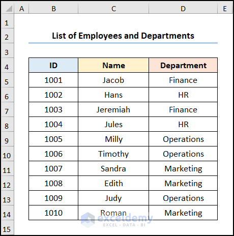
Consider the List of Employees and Departments dataset shown in cells B4:D14. This dataset includes employee IDs, their Names, and the Departments where they work. Now, let’s explore each problem and its solution with relevant illustrations.

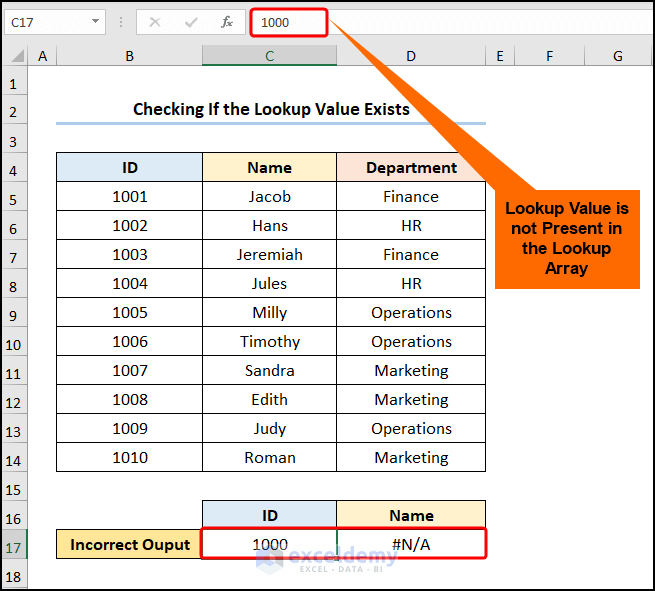
Solution 1: Checking If the Lookup Value Exists

One common cause of the VLOOKUP #N/A error in Excel is when the lookup value isn’t present in the lookup array. In such cases, the function returns an #N/A error.

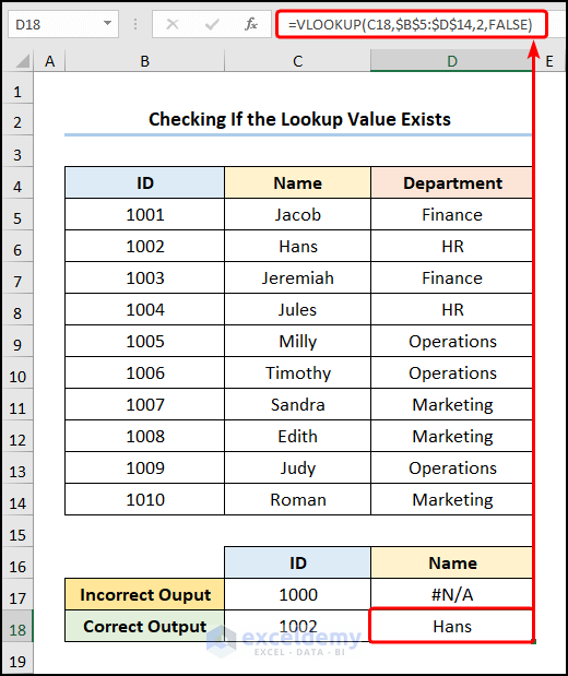
To resolve this, simply correct the value to get the desired results.

Steps:

Start by entering the correct ID number in cell C18.
Use the following formula:

=VLOOKUP(C18,$B$5:$D$14,2,FALSE)

Here, C18 represents the ID number 1002.

Formula Breakdown:

VLOOKUP(C18,$B$5:$D$14,2,FALSE) →searches for a value in the left-most column of the table array ($B$5:$D$14) and returns a value from the specified column in the same row. In this case, it matches C18 (the lookup value) from the array and retrieves the corresponding name (column 2). The FALSE argument ensures an exact match.

Output → Hans

Note: Remember to use absolute cell references by pressing the F4 key on your keyboard.

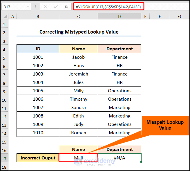
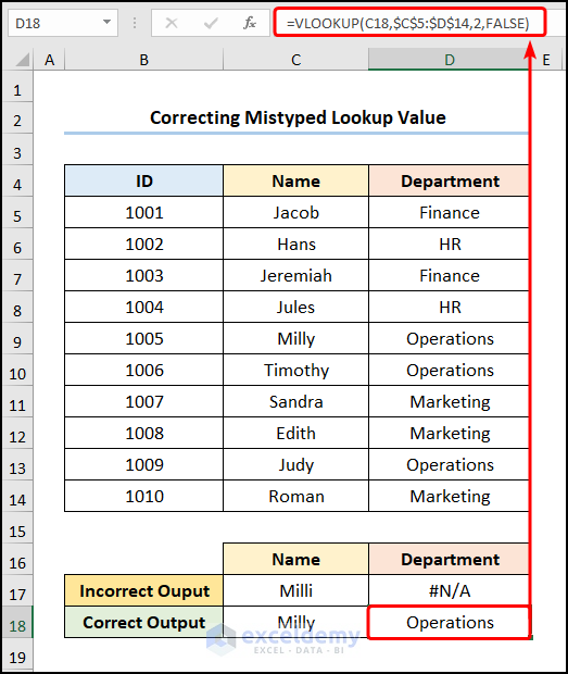
Solution 2: Correcting Mistyped Lookup Value

Another common error that frustrates users is a simple typo in the lookup value, resulting in the #N/A error. In the image below, the name “Milly” has been misspelled as “Milli.”

Thankfully, the fix is straightforward. Follow these steps:

Steps:

Enter the Correct Name:
- Start by entering the correct name in cell C18.
- Insert the following formula in cell D18:

=VLOOKUP(C18,$C$5:$D$14,2,FALSE)

For example, if the C18 cell contains the name “Milly,” this formula will return the corresponding department.

Formula Breakdown:

VLOOKUP(C18,$C$5:$D$14,2,FALSE) →searches for the lookup value (C18) in the table array ($C$5:$D$14) and retrieves the value from the second column. The FALSE argument ensures an exact match.

Output → Operations

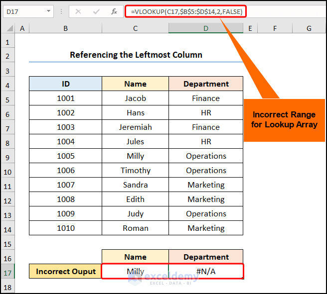
Solution 3: Referencing the Leftmost Column

Keep in mind that the VLOOKUP function cannot retrieve data from its left side. The lookup column must be the leftmost column; otherwise, the function returns the #N/A error.

Steps:

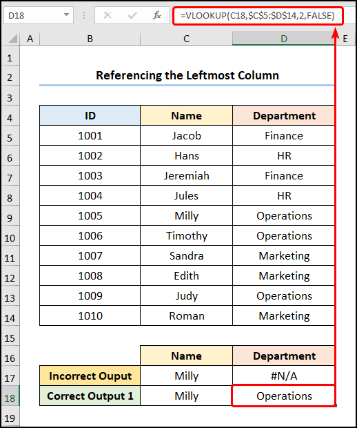
To address this, navigate to cell D18 and enter the following formula in the Formula Bar:

=VLOOKUP(C18,$C$5:$D$14,2,FALSE)

This should display the correct result, which is the department of Operations.

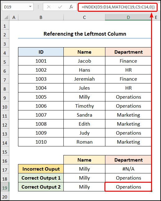
Alternative Approach: INDEX and MATCH Functions:

If you want to avoid worrying about the lookup column position, consider using the INDEX and MATCH functions.
Enter the following formula in cell D18:

=INDEX(D5:D14,MATCH(C19,C5:C14,0))

Here, the C19 cell points to the name “Milly.”

Formula Breakdown:

MATCH(C19, C5:C14, 0):
- The MATCH function returns the relative position of an item in an array that matches the given value.
- In this case:
  - C19 is the lookup value, referring to the name “Milly.”
  - C5:C14 represents the lookup array where the value is searched.
  - The 0 argument indicates an exact match.
- Output: 5
INDEX(D5:D14, MATCH(C19, C5:C14, 0)):
- The INDEX function retrieves a value at the intersection of a row and column in a given range.
- Here:
  - D5:D14 is the array argument, representing the marks scored by the students.
  - 5is the row_num argument, indicating the row location (which corresponds to the department).
- Output: Operations

Remember to use absolute cell references by pressing the F4 key on your keyboard.

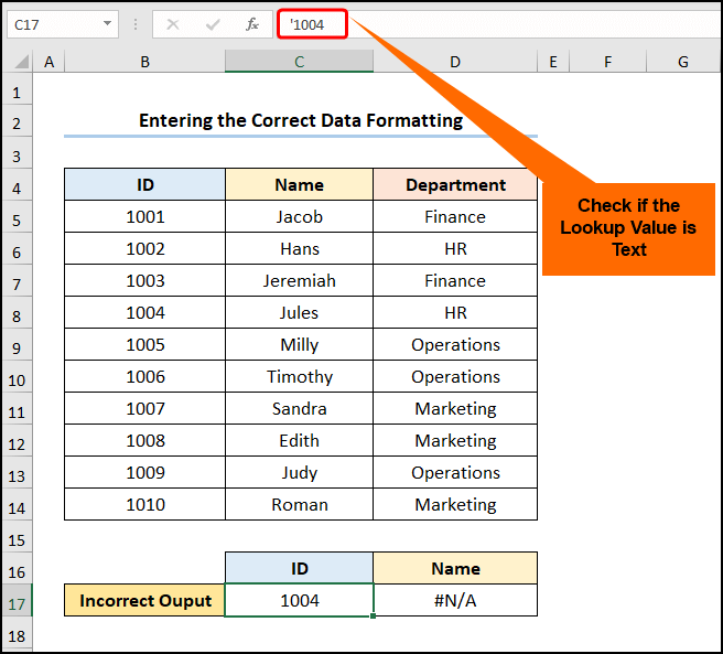
Solution 4: Entering the Correct Data Formatting

The VLOOKUP #N/A Error often occurs due to modified formatting of the lookup value during import or by mistake. Specifically, a leading apostrophe can cause the data to be interpreted as text, as shown in the screenshot below.

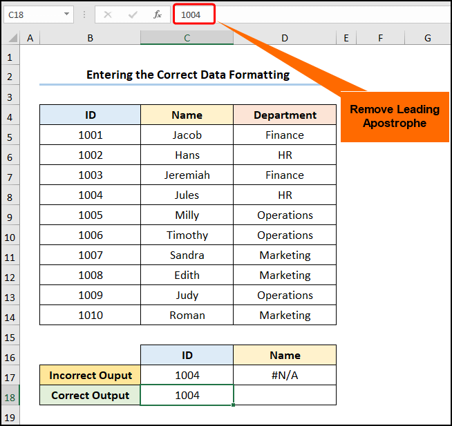
To address this issue, follow these steps:

Steps:

Remove the Apostrophe:
- Go to cell C18.
- Press the F2 key to enter Edit mode.
- Remove any leading apostrophe or extra formatting.

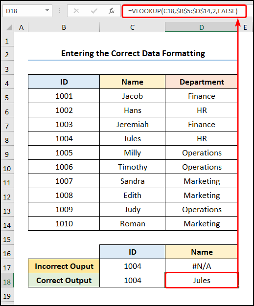
Calculate the Correct Output:
- In cell D18, use the following formula:

=VLOOKUP(C18,$B$5:$D$14,2,FALSE)

For example, if the C18 cell contains the ID number 1004, this formula will return the corresponding name (e.g., Jules).

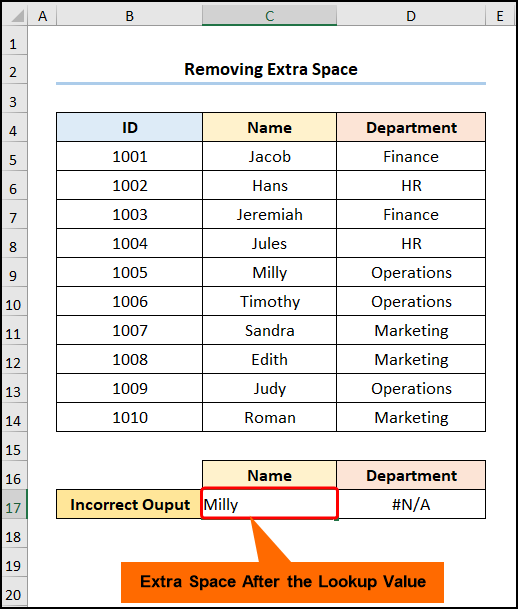
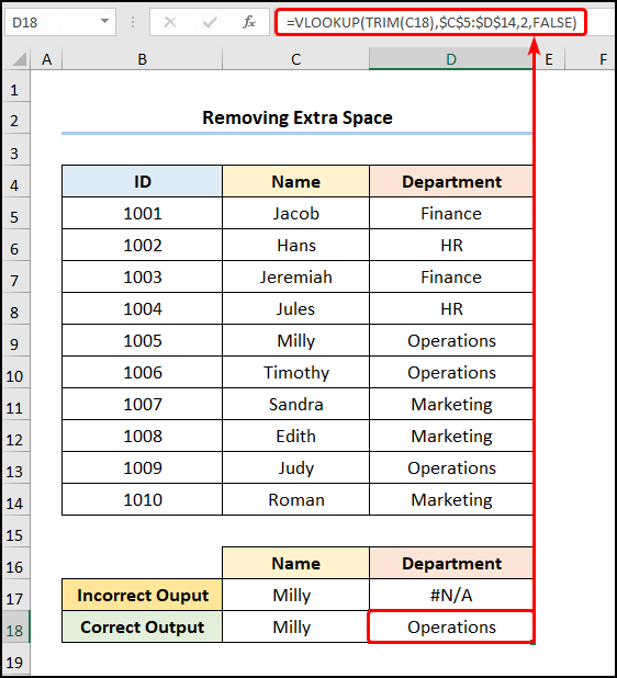
Solution 5: Removing Extra Space

The VLOOKUP formula may not work correctly if the lookup value contains extra spaces. To resolve this, we’ll use the TRIM function to eliminate any additional spaces within the lookup value.

Steps:

Remove Spaces:
- Enter the D18 cell.
- Type the following expression:

=VLOOKUP(TRIM(C18),$C$5:$D$14,2,FALSE)

The TRIM function removes all but single spaces from the text in the C18 cell (e.g., “Milly “).

Formula Breakdown:

TRIM(C18) removes excess spaces after the text.
The modified formula becomes:

VLOOKUP(“Milly”,$C$5:$D$14,2,FALSE)

Here, “Milly” (lookup_value argument) is matched from the table array ($C$5:$D$14). The 2 (col_index_num argument) represents the column number of the lookup value, and FALSE ensures an exact match.

Output → Operations

Remember to use absolute cell references by pressing the F4 key on your keyboard.

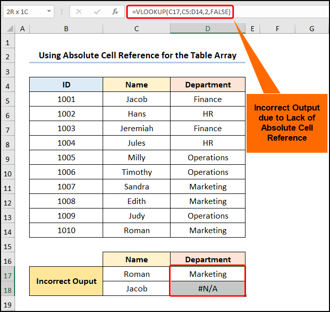
Solution 6: Using Absolute Cell Reference for the Table Array

Another potential cause of the VLOOKUP #N/A Error is neglecting to use Absolute Cell References for the table array. When you copy the formula using the Fill Handle tool, it shifts the cells of the lookup array. Consequently, the function may fail to match the lookup value within the given array.

Follow these steps to address this issue:

Steps:

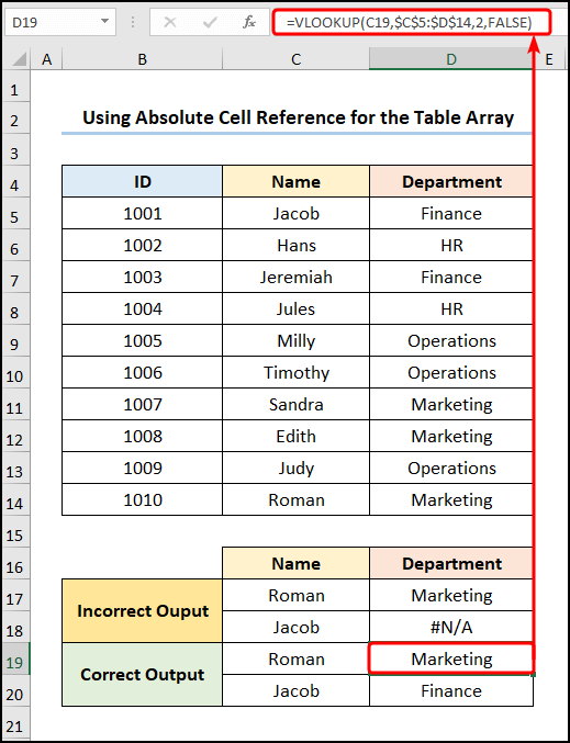
Apply Absolute Cell Reference:
- Go to cell D18.
- Use the following formula:

=VLOOKUP(C19,$C$5:$D$14,2,FALSE)

For example, if the C19 cell contains the name Roman, this formula will return the corresponding department.

Note: Press the F4 key on your keyboard to lock in the $C$5:$D$14 cell references.

Final Thoughts:
- While we strive for perfection, our world isn’t flawless! The methods mentioned above are all potential fixes for the VLOOKUP #N/A Error.
- If the problem persists, consider reaching out to Microsoft Support. They have Excel experts who can provide tailored solutions for your specific issues.

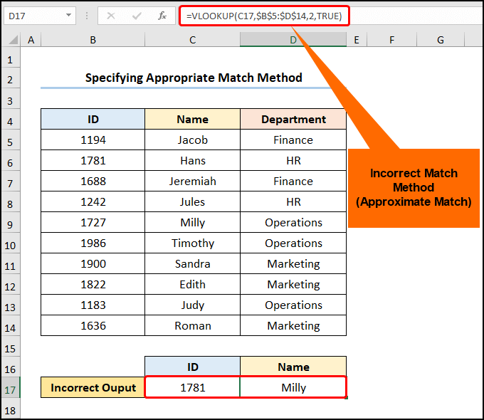
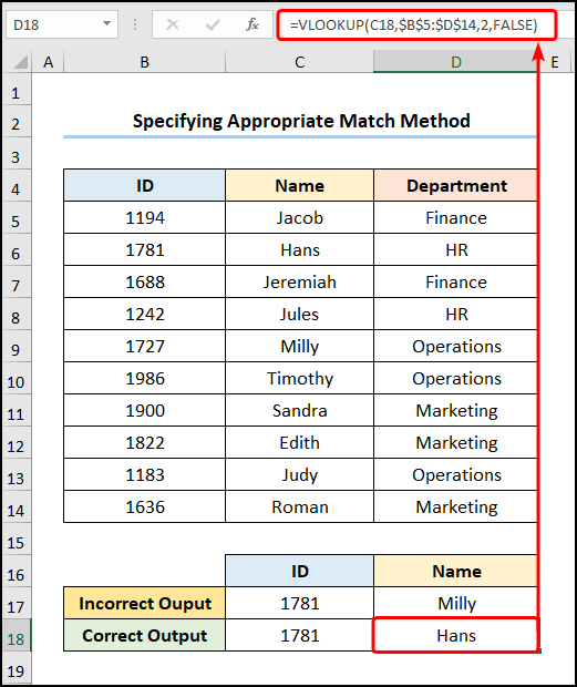
Specifying Appropriate Match Method in VLOOKUP Formula

Additionally, specifying the wrong match method in the VLOOKUP function can lead to incorrect output even if the data exists. Specifically, using the TRUE argument results in an approximate match condition, which matches the nearest value and may return an erroneous result.

In the following section, we’ll discuss how to troubleshoot this issue:

Steps:

Exact Match Criteria:
- Go to the D18 cell.
- Enter the following equation:

=VLOOKUP(C18,$B$5:$D$14,2,FALSE)

Here, the FALSE argument ensures an exact match in the VLOOKUP function.

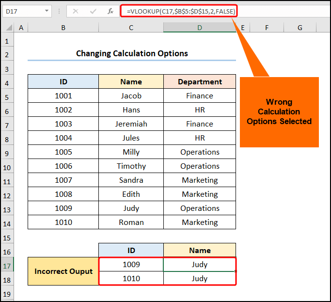
What to Do If VLOOKUP Function Is Not Returning Correct Value

You may need to verify whether Excel’s Calculation Options are set to Manual, as this setting can cause the VLOOKUP function to produce the same result when copied into cells below. Typically, this feature is designed to prevent unnecessary calculations and thereby avoid slowing down the computer. However, not reverting to the default Automatic option can lead to issues, as illustrated in the screenshot below.

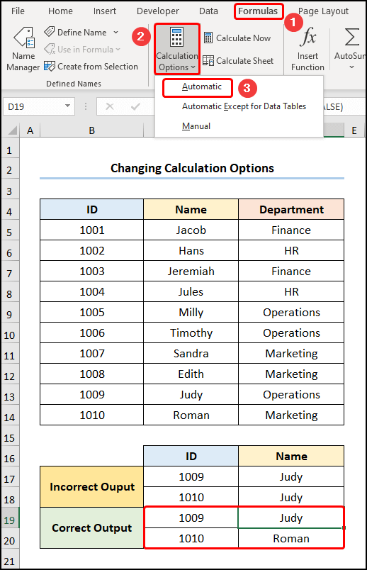
Steps:

Go to the Formulas tab and click on the Calculation Options drop-down menu.
Ensure that the Automatic option is selected.
You should see the correct output, as depicted in the image below.