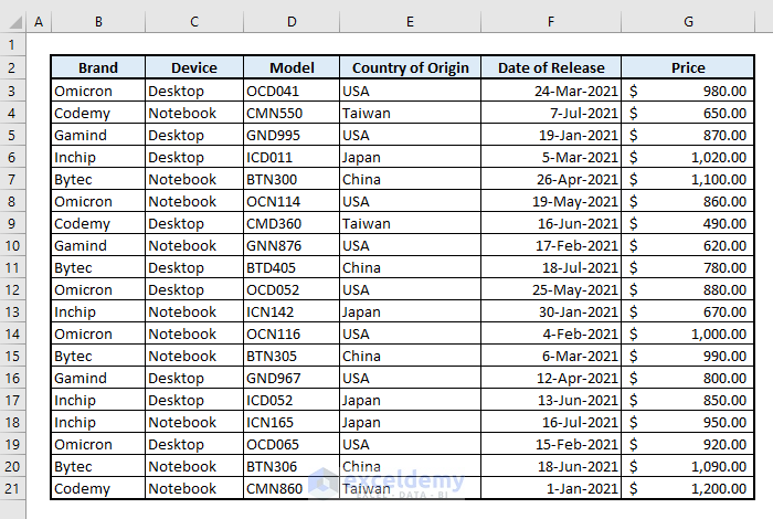
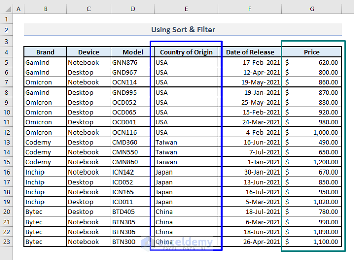
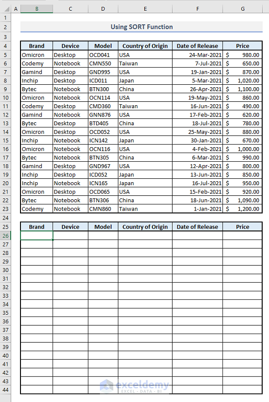
We will use the sample dataset below for illustration.
Watch Video – Sort Multiple Columns in Excel
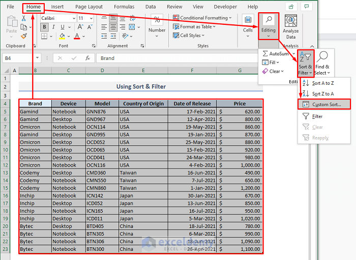
Method 1 – Using Sort & Filter Command to Sort Multiple Columns
We want to add 2 criteria for sorting columns in our dataset. We’re going to sort the names of the countries of origin by the order of Z to A. After that, the device prices will be sorted by smallest to largest.
Step 1:
➤ Select the entire table data first.
➤ Go to the Home ribbon, select the Custom Sort command from the Sort & Filter drop-down in the Editing group of commands. A dialog box will open.
Step 2:
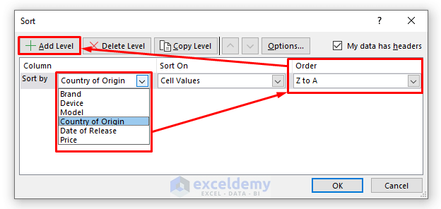
➤ Tap on the Sort by drop-down & select Country of Origin.
➤ Change the order by Z to A from the Order drop-down.
➤ Click on Add Level to assign another criterion.
Step 3:
➤ Select Price from the next drop-down.
➤ Change order from Smallest to Largest.
➤ Press OK.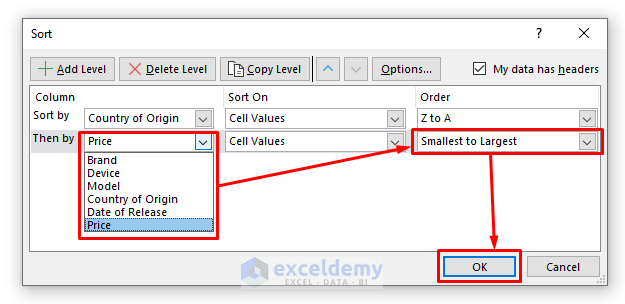
You’ll have your sorted data for all columns at once. In Column G, the prices are sorted based on the orders of the country names as we’ve assigned the order for prices as the secondary criteria for sorting.
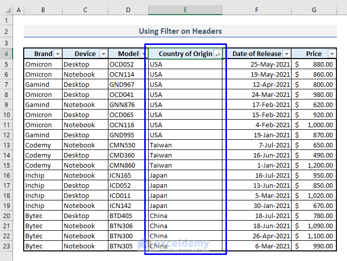
Method 2 – Assigning Filter Options on the Table Headers
Step 1:
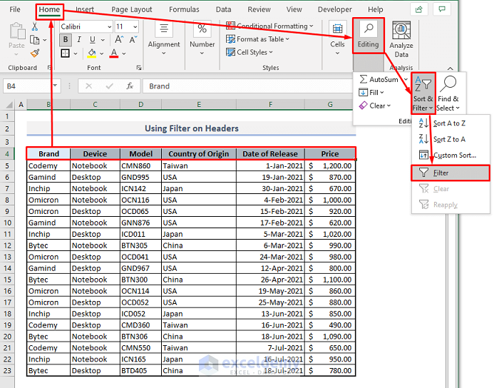
➤ Select all the headers of the table first.
➤ Under the Home tab, choose Filter command from the Sort & Filter drop-down in the Editing group of commands. You’ll find the Filter buttons on your table headers.
Step 2:
➤ Click on the Country of Origin drop-down.
➤ Select the order- Sort Z to A.
➤ Press OK.
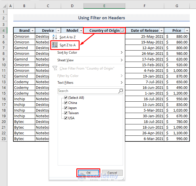
You’ll get the sorted columns based on the countries of origin.
Method 3 – Conditional Formatting to Sort Multiple Columns
If you want to sort your data or columns by highlighting with colors or symbols you have to choose Conditional Formatting. This method doesn’t rearrange data but visually highlights rows based on sorting criteria. Let’s assume that we want to sort the column for Date of Release by highlighting the data.
Steps:
➤ Select the entire column you want to highlight (example, Date of Release).
➤ Go to the Home tab, click Conditional Formatting, and Color Scales. From the drop-down list, choose the Green-White or any other color scale you prefer. You’ll be shown a preview of that color scale in your assigned column.
➤ Press Enter.
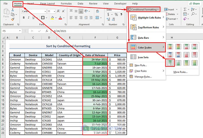
The assigned column will be highlighted with Green-White color scales where the full green part denotes the latest dates and light green or white ones are for older dates.
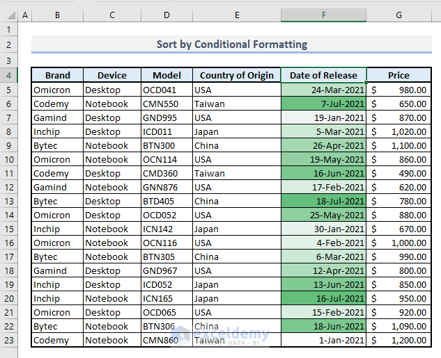
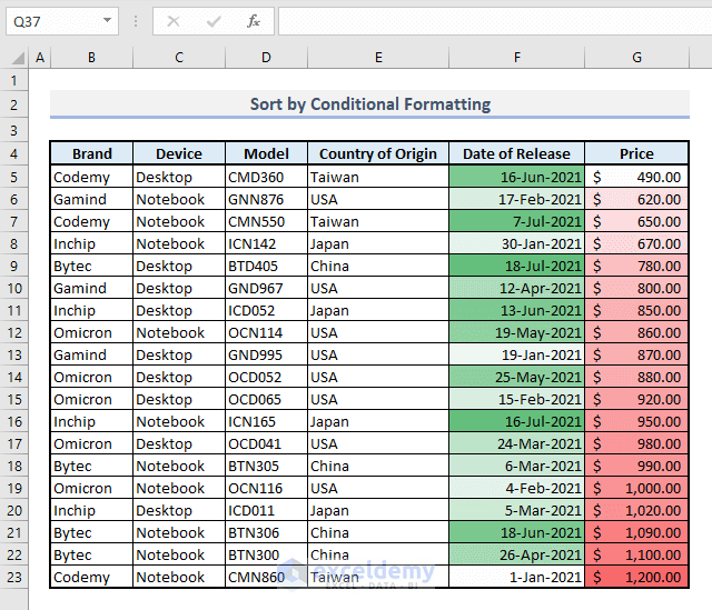
You can sort the column for prices too with similar or another range of color scales. Here, the prices are sorted in an ascending order & then if you use color scales, it’ll look the image below.
Sorting by color scales depends on the available numerical data. If you want to sort text strings in a column or a row, then you have to look for another method or customize the selected data from Conditional Formatting.
Method 4 – Inserting SORT Function to Sort Multiple Columns
- Objective of the Function:
Sorts a range of an array.
- Syntax:
=SORT(array, [sort_index], [sort_order], [by_col])
- Arguments:
array- Range of data or cells that you want to sort.
[sort_index]- Column or row number that’ll be sorted.
[sort_order]- Ascending(1) or Descending(-1) order.
[by_col]- You have to choose whether the sorting will be done by column or by row.
In this image, another table has been added under the first one where we’ll apply the SORT function based on the data in the original table.
Steps:
➤ Select the output Cell B26 & type:
=SORT(B5:G23,6,-1,FALSE)➤ Press Enter and you’ll find the sorted columns in the second table.
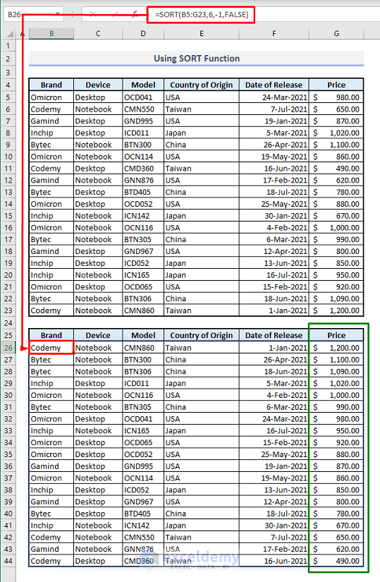
We’ve only sorted the prices here by largest to smallest. Inside the function, the 1st argument is B5:G23 which is the selected range of data to be sorted. Here sort_index or column number has been chosen as 6 since the 6th column represents the prices. ‘-1’ in the 3rd argument means, we’re sorting the data in descending order. In the 4th argument, the logical function FALSE has been chosen to assign the sorting by rows, not by columns.
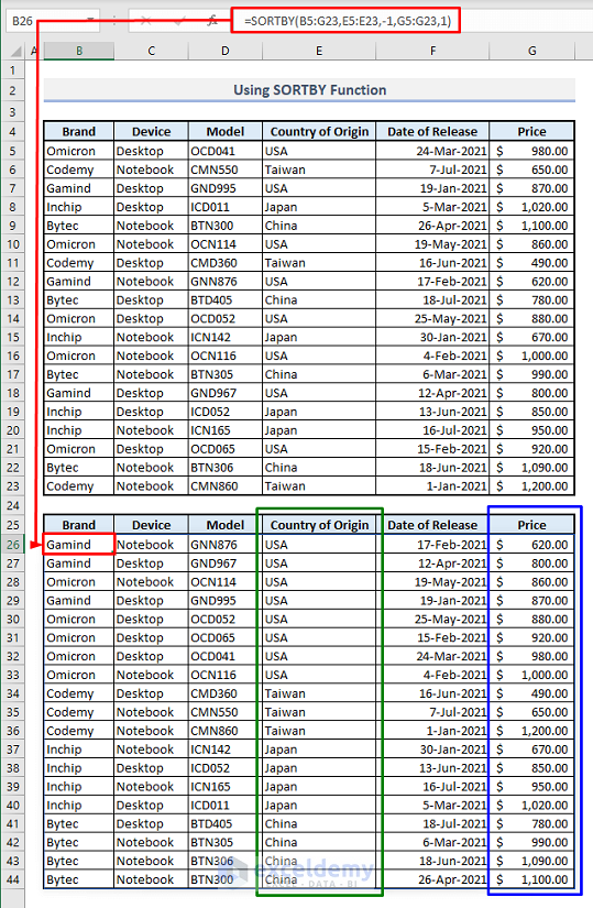
Method 5 – Applying SORTBY Function to Sort Multiple Columns
By using the SORTBY function, you can add multiple criteria for sorting columns. The syntax of this formula is:
=SORTBY(array, by_array1, [sort_order1], [by_array2], [sort_order2])
Based on our dataset, we’ll sort the column for Country of Origin first, and then the prices will be sorted by smallest to largest.
Steps:
➤ Select Cell B26 and type:
=SORTBY(B5:G23,E5:E23,-1,G5:G23,1)➤ Press Enter and you’ll be shown the sorted array in the second table.

Inside the function, 1st argument is the selected array of data that has to be sorted. The 2nd and 3rd arguments are the range of cells- E5:E23 & -1 respectively. It means the text data in Column E will be sorted by the alphabetical order of Z to A. These two arguments combine the first criteria for sorting. The second criteria consists of the arguments G5:G23 and ‘1’ which indicates that the prices in Column G will be sorted by smallest to largest.
How to Sort Multiple Columns in Excel: Knowledge Hub
- How to Sort Two Columns to Match in Excel
- How to Sort Alphabetically with Multiple Columns in Excel
- How to Sort Multiple Columns in Excel Independently of Each Other
- How to Sort Columns in Excel Without Mixing Data
<< Go Back to Sort in Excel | Learn Excel
Get FREE Advanced Excel Exercises with Solutions!
