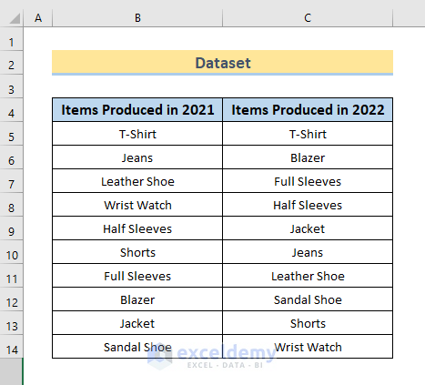
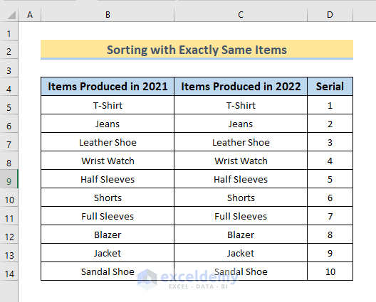
We will use a dataset that includes Items Produced in 2021 and Items Produced in 2022 of a company.
Method 1 – Sort Two Columns to Match with Exactly the Same Items
The two columns contain the same items but in different orders. We will sort the second column to match the first column.
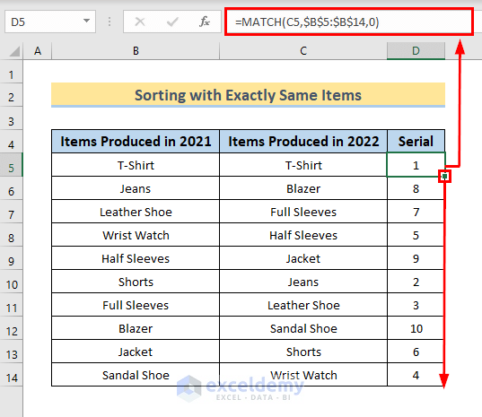
- Make a new column Serial and insert the following formula in Cell D5.
=MATCH(C5,$B$5:$B$14,0)- Press Enter.
- Use the Fill handle to copy the formula in the cells below.
- Select the range of cells C5:D14.
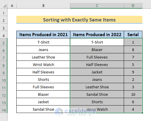
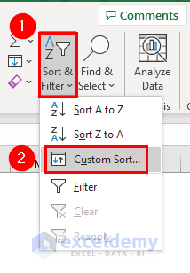
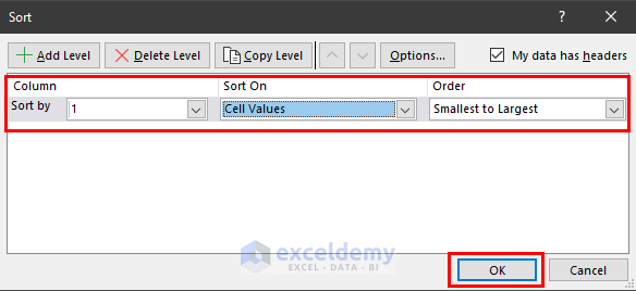
- Select Sort & Filter and choose Custom Sort in the Home tab.
- In the Sort window, choose 1 (value in Cell D5) in the Sort by section, Cell Values in Sort on section, and Small to Largest in the Order section.
- Press OK.
- The second column is sorted according to the first column.
Read More: How to Sort Multiple Columns in Excel Independently of Each Other
Method 2 – Sort Two Columns to Match with Partially Matched Items
Case 2.1 – If the First Column Has All Items of the Second Column
Part 2.1.1 – Sorting in the Same Location
- Create a new column Serial and use the following formula in cell D5.
=MATCH(C5,$B$5:$B$14,0)- Press Enter and use the Fill Handle to copy the formula down to Cell D10.
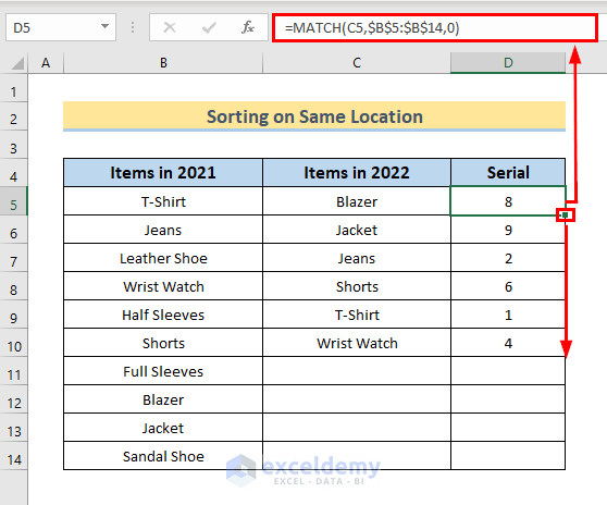
In the formula, the MATCH function has arguments C5 as the matching value, $B$5:$B$14 is the range for matching and 0 denotes exact matching.
- Use the following formula in Cell D11.
=FILTER(ROW(A1:A10),COUNTIF(D5:D10,ROW(A1:A10))=0)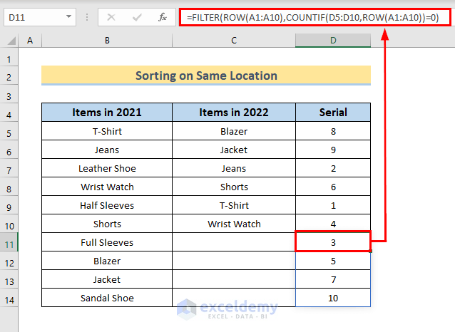
- We have taken ROW(A1:A10) because the first column consists of a total of 10 items (B5 to B16). If your first column consists of 50 items, use ROW(A1:A50).
- D5:D10 is the range in the new column which was filled before applying this formula.
Note: The formula is in array form so press Ctrl + Shift + Enter for versions of Excel other than Excel 365.
- Copy the cell values from D5:D14 that contain the serial number.
- Paste them as values.
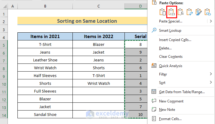
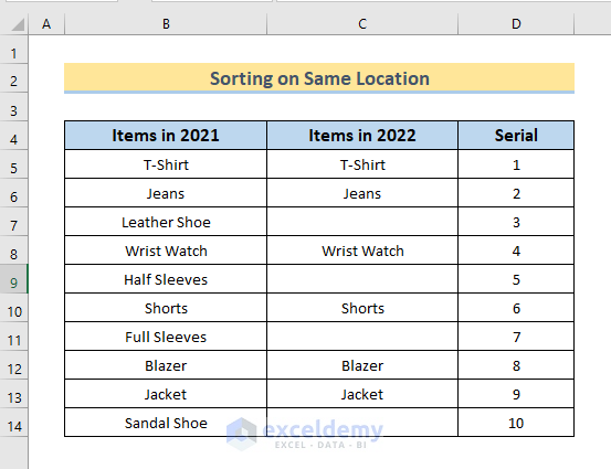
- Sort Column D and Column C following the procedures in Method 1.
- We will see the second column sorted according to the first column.
Read More: How to Sort Alphabetically in Excel with Multiple Columns
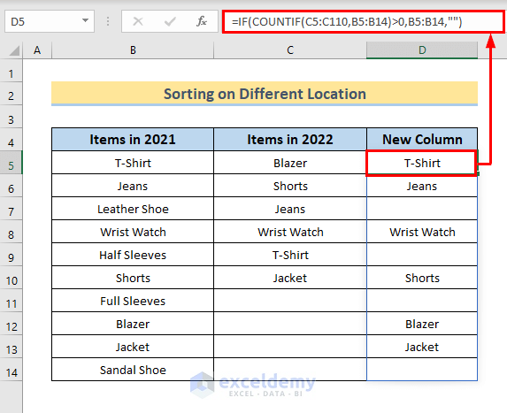
Part 2.1.2 – Sorting in a Different Location
- Create a New Column and use the following formula in cell D5.
=IF(COUNTIF(C5:C110,B5:B14)>0,B5:B14,"")- Press Enter.
- The second column’s data is sorted according to the first column’s data in the New Column.
Note: we have used an array formula so press Ctrl + Shift + Enter for other versions of Excel.
Read More: Sorting Columns in Excel While Keeping Rows Together
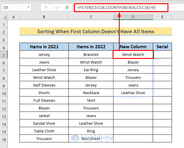
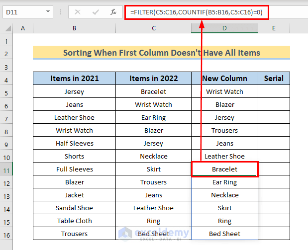
Case 2.2 – If the First Column Doesn’t Have All Items of the Second Column
- Insert two additional columns New Column and Serial after the two columns.
- Use the following formula in Cell D5.
=FILTER(C5:C16,COUNTIF(B5:B16,C5:C16)>0)- Press Enter for Excel 365 or press Ctrl + Shift + Enter for previous versions.
- The first empty cell below the array formula result is Cell D11.
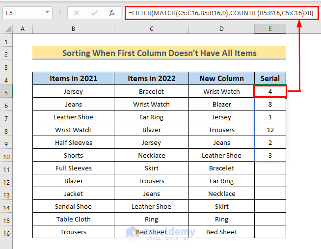
- Use the following formula in the cell.
=FILTER(C5:C16,COUNTIF(B5:B16,C5:C16)=0)- Press Enter for Excel 365 or press Ctrl + Shift + Enter for previous versions.
- Use the following formula in Cell E5.
=FILTER(MATCH(C5:C16,B5:B16,0),COUNTIF(B5:B16,C5:C16)>0)- Press Enter for Excel 365 or press Ctrl + Shift + Enter for previous versions.
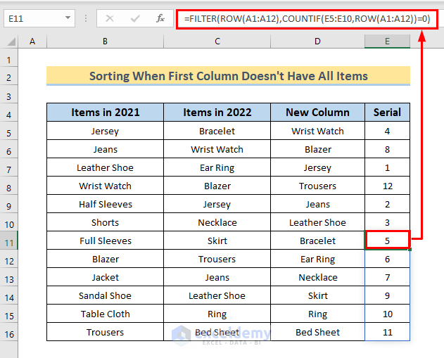
- Use this formula in Cell E11 (where the list ends).
=FILTER(ROW(A1:A12),COUNTIF(E5:E10,ROW(A1:A12))=0)- Press Enter for Excel 365 or press Ctrl + Shift + Enter for previous versions.
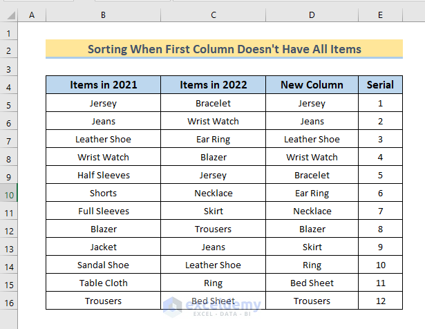
- Copy the data from Column D and Column E and paste only values in the same place.
- Sort Column D and Column E just like in Method 1 and you will get the sorted data in the New Column.
How to Find If the Data of Two Columns Match in Excel
- Use the following formula in Cell D5.
=IFERROR(VLOOKUP(C5,$B$5:$B$15,1,0),"Data Doesn't Match")- Press Enter and use the Fill Handle to copy the formula in the cells following.
- We will see matched data in the cells. If the data doesn’t match, the Data Doesn’t Match text will appear in the cell.
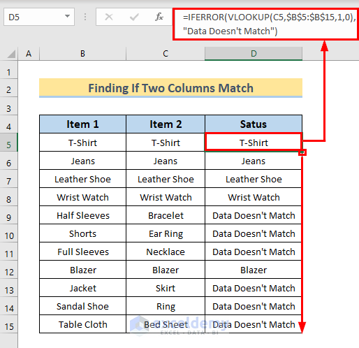
The VLOOKUP function checks the data from Cell C5 and from range $B$5:$B$15 and gives that data as output which is taken as an argument for the IFERROR function. If data is not found by the VLOOKUP function, the IFERROR function gives the output Data Doesn’t Match as it is in the argument.
Download the Practice Workbook
Further Readings
- How to Sort Columns in Excel Without Mixing Data
- Sort Alphabetically in Excel and Keep Rows Together
<< Go Back to Sort Columns in Excel | Sort in Excel | Learn Excel
Get FREE Advanced Excel Exercises with Solutions!

It help me so much, I was strugle at 2. Matching Two Columns with Not Exactly the Same Items. Now, I know how to done it, thanks to you, cheers.
Hey,
Thank you for the helpful article!
I have one question to ask to “2. Matching Two columns with Not Exactly the Same Items”:
If i want to sort the data in the second coloumn (items produced in 2020) to match not only data added to the coloumn: items produced in 2019 (as you do here), but also data added to a coloumn more, called: items produced in 2018. and 1) the 2018 coloumn have the same data as the 2019 coloumn have, 2) their data are placed at the same rows and 3) the 2018 coloumn have some empty cells (for instance while 2019 coloumn have a cell with the text “monkey”, the cell beside (which belongs to 2018 coloumn) is empty. So How do i sort the data from the coloumn: items produced in 2020) not only to match one coloumn (items produced in 2019) but to match two coloums?(items produced in 2018 and items produced in 2019)
Thank you in advance.
Anton
Hello Anton,
First of all, you have to create three columns including items produced in 2018. Here, we need to paste the same value as items produced in 2019. Just one or two blanks in there.
Then, take a new cell and write down the following formula.
=IF(COUNTIF(D5:D12,B5:C19)>0,B5:C19,””)
Here, the range becomes (D5:D12 as the column of items produced in 2020 changes. Then, the criterion becomes B5:C19. Here, it follows if the condition match for both cells then it will return the value. Otherwise, it returns blank. After that, press Ctrl+Shift+Enter as it is an array formula.
Here, you can see, that the product Trousers is available in 2019 and 2020. but, we give criteria for products in 2018 and 2019. As they don’t find trousers in 2018, that’s why you won’t get them in the result. So, you will get the products that are available in both 2018 and 2019.
Hi,
Using your case 2 example, how would you align the items that do not match with a blank cell on both sides (instead of having them on the same row). E.g. blank – skirt & jacket – blank
Many thanks
Hello,
First of all, download the Practice Workbook for better understanding.
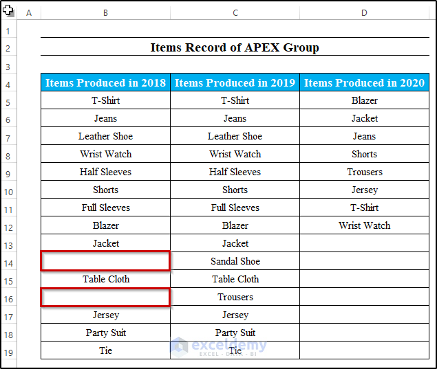
I think you’ve talked about the following phenomena. Let’s see the following image.
Now, you want to match the items in Column 2020 with the items in Column 2019.
For this, copy the cells in the B5:B12 range.
Then, paste them in the E5:E12 range.
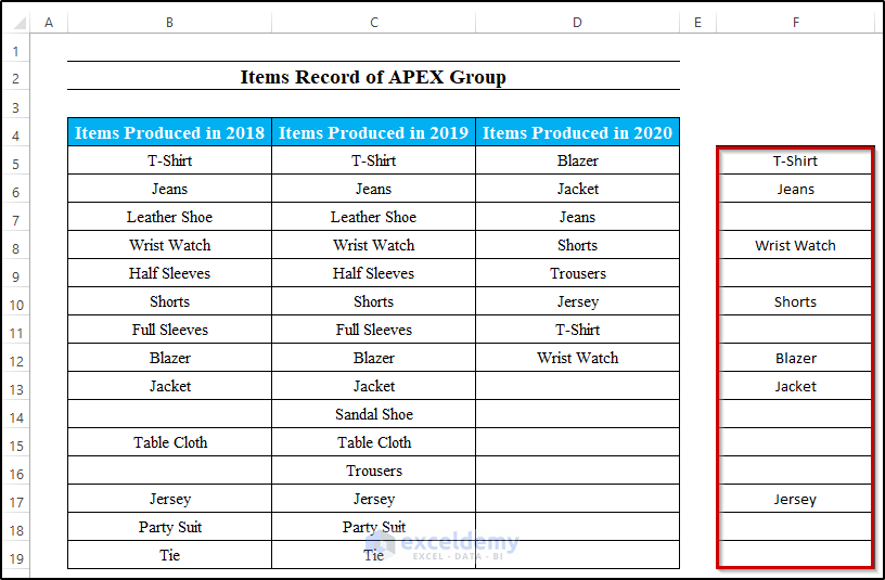
After that, go to cell F5 and enter the following formula.
=IF(COUNTIF(C5:C12,B5:B12)>0,B5:B12,"")As usual, press ENTER.
Note: It’s an array formula. If you are using Microsoft Excel 365 then you can easily run the formula by pressing the ENTER key. Otherwise, you have to tap the CTRL+SHIFT+ENTER keys simultaneously to make the formula work.
Hope that will work for you. Follow our blog Exceldemy to learn more about Excel.